Sparse Virtual Shadow Maps
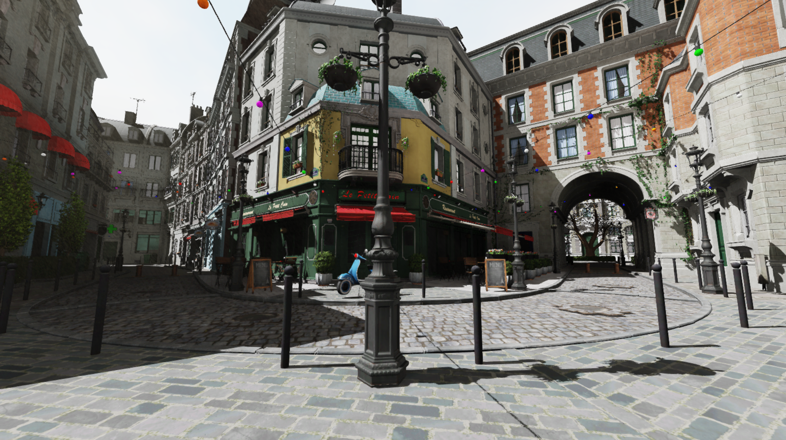
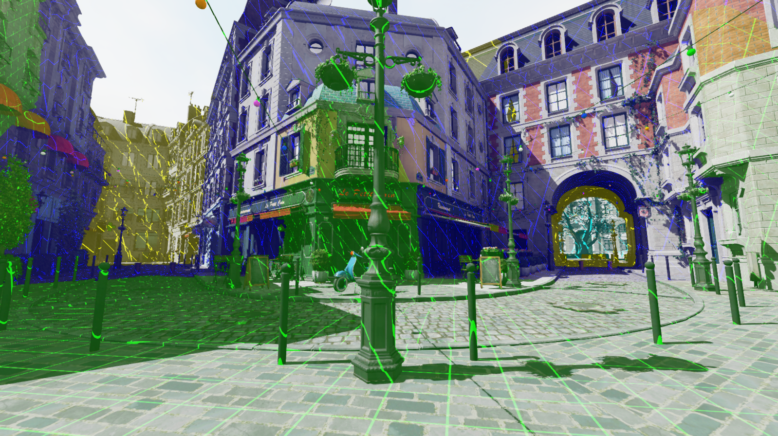
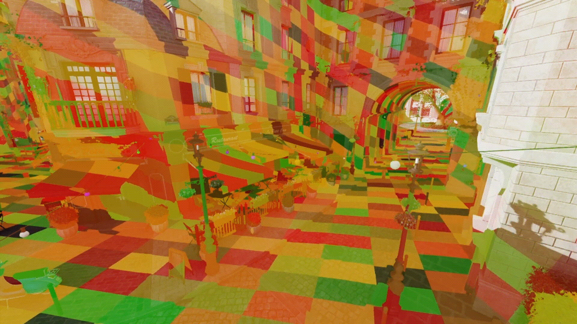
The top is the Bistro scene rendered with multiple 8K resolution sparse virtual shadow maps. The bottom is a visualization of the virtual memory pages (squares) where each color represents a different shadow clipmap/cascade.
Feedback is greatly appreciated!
Last edited: Nov 2, 2023
Collaborators
This was developed in loose collaboration with:
Table of Contents
- Collaborators
- Table of Contents
- Introduction
- Motivation and Comparison
- Foundations
- Physical Memory Format
- Method Overview
- Modifying Virtual Viewport Matrices
- Mapping Virtual Memory to Physical Memory
- Selecting Clipmaps
- Cache Invalidation Events
- Allocation Strategy
- Physical Memory Limits
- Shadow Render Budget
- Hardware Shadow Filtering
- Post-Processing Effects
- References
Introduction
This post goes through the high-level steps needed to create a virtual memory system for realtime shadows. This was inspired by Unreal Engine 5’s virtual shadow maps. Directional lights are the only ones considered here, but it is possible to extend the system to support other light types such as point or spotlights.
The directional shadows make use of clipmaps for incremental updating of the shadowmaps and handling multiple different cascades. Each clipmap cascade can be set to very high virtual resolutions such as 4K, 8K or 16K.
Sparsity
Part of the strength of this method comes from its ability to represent shadows using sparse textures. If nothing is currently present in one of the clipmap cascades, that cascade’s memory footprint and processing overhead can be reduced to almost nothing.
Virtual
This system replaces normal shadow map uv coordinates with virtual uv coordinates. To either write to or read from the shadow maps, virtual uv coordinates have to be translated to physical uv coordinates. The actual physical memory pool can be much smaller than what the virtual uv coordinate space would suggest. Conceptually this is extremely similar to virtual memory systems in modern operating systems.
Caching
As the camera moves around the scene, new virtual pages become visible and are rendered incrementally. Previously rendered pages that are still visible and haven’t changed can be reused from frame to frame to save on performance. For either debugging purposes or to make it easier to build an initial prototype, caching can be disabled or skipped in favor of being added later.
Motivation and Comparison
The motivations for using this approach fall into two categories:
- Significant increase in shadow map resolution while maintaining highly configurable (even dynamic) performance costs
- Provide the ability to cover massive world distances with a single shadow technique
Comparison to Cascaded Shadow Maps
An important aspect mentioned in the introduction is that if a cascade doesn’t have much geometry inside of it, processing overhead and memory footprint for that cascade can be reduced close to 0. This opens the possibility of maintaining 10, 15 or even 20 cascades. In addition, if the virtual resolution is set to 8K or 16K, every cascade gets its own 8K or 16K virtual shadow map. This allows for high quality, consistent shadows that cover huge world distances.
Standard cascaded shadow maps (CSMs) struggle to handle this without heavy optimization. In many ways sparse virtual shadow maps are an extension of CSMs with the optimizations required to improve memory usage, increase resolution, cover even larger max distances, and avoid duplicate shadow reprocessing for data that hasn’t changed since last frame.
Other Light Types
Even though this article focuses on directional lights, it is possible to virtualize other light types such as point or spotlights. To do this, the shadow maps for each light which use fixed texture allocations will be replaced with virtual shadow textures that are mostly sparse. For point lights this would result in 6 virtual textures (virtual cubemap) each with virtual mipmaps while spotlights would only need 1 virtual texture with virtual mipmaps. Physical backing memory for the virtual shadow textures of all the different light types can come from the same shared texture memory pool.
Foundations
This technique is built off two core foundations: sparse virtual texturing and clipmaps.
Sparse Virtual Texturing
Helpful resources:
With regular virtual memory, all addresses used by a user mode application are virtual addresses. When the memory needs to be used in some way, the OS must translate the virtual addresses into physical addresses. Using this system, some of the bits of the virtual address are used as an offset into a translation (page) table, and that entry in the page table is used to determine where in physical memory to go. Each entry in the page table represents a physical page/block of memory with a fixed size (ex: 4 kb).
An important part of a virtual memory system is that it is not required to always have everything available in RAM. Parts that aren’t needed can be paged out to secondary storage and kept there until requested. When a process makes a request to access a piece of memory that is either out of date or not present in RAM at all, this is known as a page fault. When this happens, it is the job of the OS to handle it by making sure that the memory the process is trying to use is present and up to date. Once this is done the process can resume execution.
Sparse virtual texturing uses the same approach. For this to work, each physical page of memory is a 2D block of size 128x128 texels (or some other power of two supported by the hardware). For an 8K x 8K virtual texture, this would result in 64x64 page table entries. This 64x64 grid is our version of the page table.
Like with other virtual memory systems, sparse virtual texturing only maintains the minimum amount of texture data in memory for the application to continue normally. It does this by analyzing the current camera view of the scene to determine what is needed verses what can be left unallocated.
At runtime, shaders will use virtual coordinates rather than physical coordinates. These virtual coordinates are translated to physical coordinates using the page table. When the data that the virtual coordinates reference is not currently resident in physical memory, this results in a page fault. Some mechanism (such as readback SSBO) needs to be used to tell the CPU to perform an allocation and prepare the physical memory for use.
Sparse virtual shadow mapping borrows all these ideas with one exception: page faults don’t require us to read from secondary storage. Instead, page faults represent a piece of memory that we need to render shadows into so that the shaders can compute shadowing or post processing effects properly.
Clipmaps
Helpful resources:
Directional light shadow maps are represented by a series of expanding rings around the player camera known as clipmap rings. Conceptually they are similar to cascades in cascaded shadow maps.
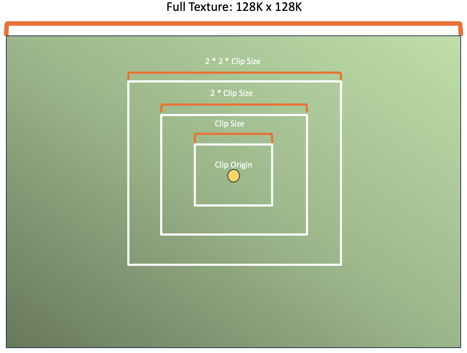
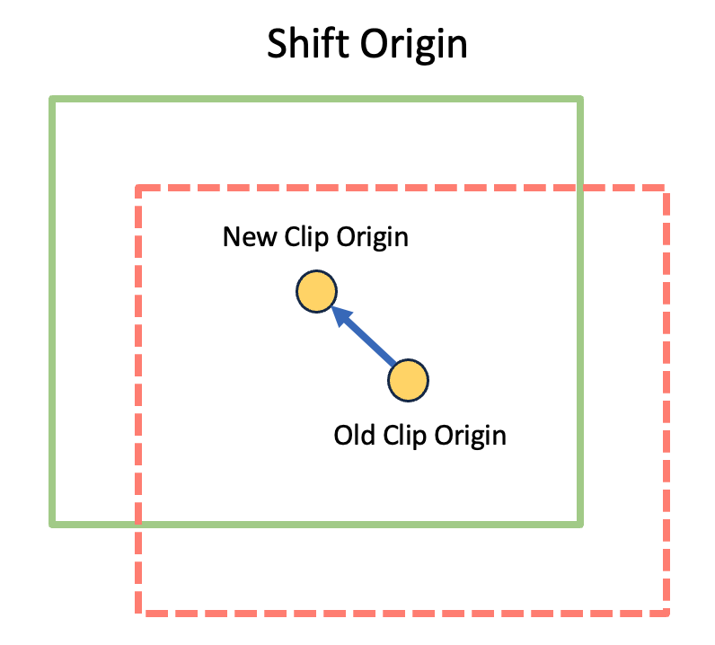
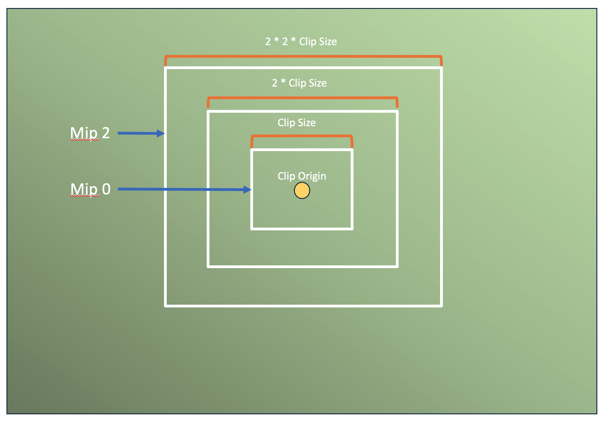
A clipmap is an incrementally updatable, fixed-size texture region that is meant to represent a subset of a full texture’s mipmap chain. A clipmap is defined by a clip origin and a clip size. Together these two determine which part of the full texture that the clipmap currently represents. As the clip origin shifts from frame to frame, new data is streamed in and old data streamed out along the borders of the texture.
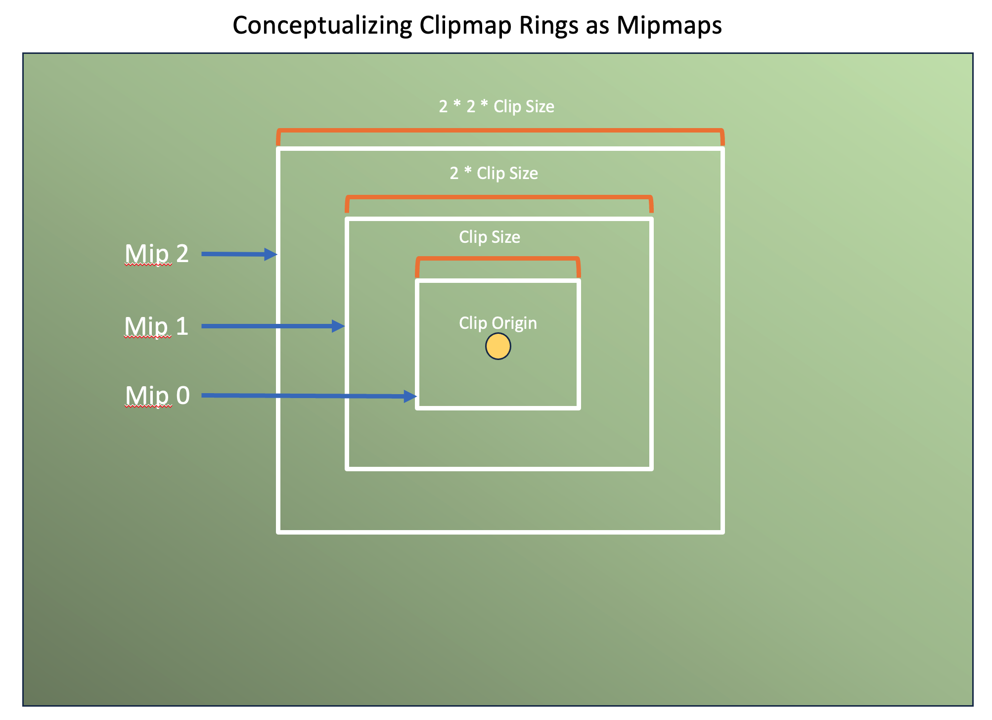
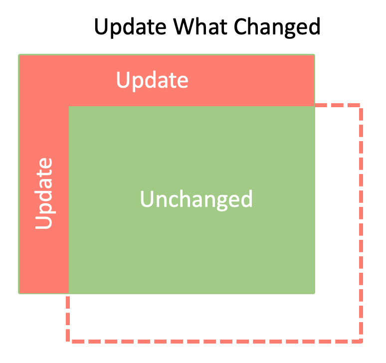
Each clipmap ring is required to cover double the area of the previous clipmap ring. This means that each successive ring is coarser/lower resolution than the previous since the memory footprint remains the same for each ring regardless of how much area they cover. Because coarser clipmap rings fully overlap finer clipmap rings, we can conceptualize them as being a version of texture mipmapping.
When sampling from a clipmap, we select the most detailed (lowest clipmap ring) that’s available. If not available, we clip to the next best fit. Later on this article will discuss the configurable shadow render budget which can lead to situations where we have to fallback to lower resolution data while higher resolution data is processed over multiple frames.
For shadow mapping, we can imagine that the “true” shadow map is something massive like 128K x 128K or more. As the player camera moves around, we will shift the clip origin to match the new camera location and update only the parts that changed.
The arrow in the above picture is a 2-component motion vector. If converted to NDC space, it can be used to project from current frame to previous frame or vice versa in order to determine which virtual pages have changed.
The new data wraps around and is written to the region where the old, no longer needed data used to be.
It’s important to keep in mind that with the virtual memory system this article outlines, each clipmap has access to the full virtual texture resolution. It is as if each clipmap has its own 4K, 8K or 16K texture even though most of it is not backed by physical memory.
Physical Memory Format
The physical backing memory can be created as a 32-bit floating point texture. Depending on which operation is being done (read vs write), the texture may be converted to a compatible format that is more convenient for us to use. The main example in this article is during shadow map rendering where we bind it as a 32-bit unsigned integer image in order to gain access to image atomic min/max.
Method Overview
This is a brief overview of all the steps required to render shadows for a single frame. The next sections will go over the steps in a lot more detail.
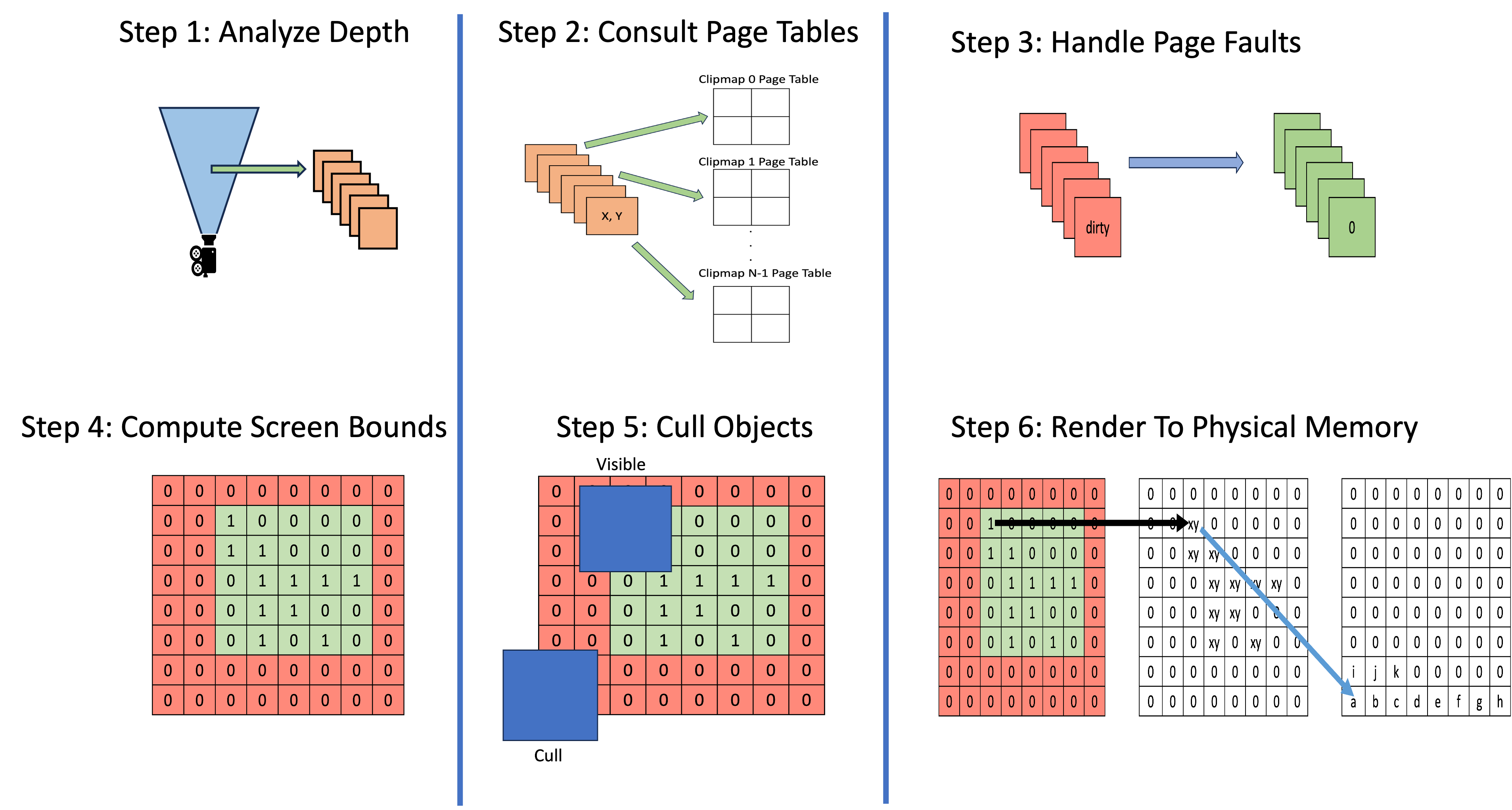
Step 1: Analyze Depth Buffer
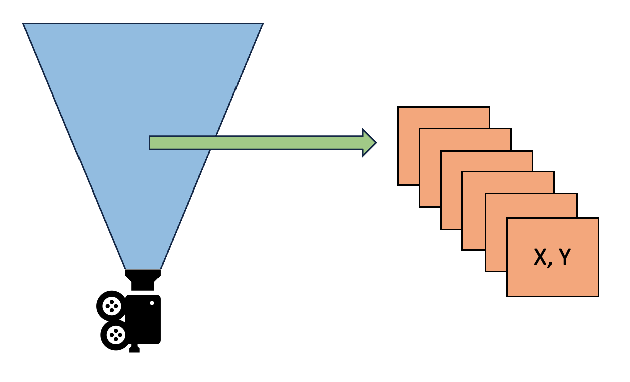
The process starts after the main camera’s depth buffer has been generated. For each depth sample, first transform it to world space coordinates. The light’s view-projection matrix is then used to convert from world space to NDC and then to virtual texture coordinates. Once the virtual texture coordinates have been computed they can be wrapped around to the nearest page table entry. This page table entry is what is marked as needed for this frame. The reason we need to wrap around is because the lightViewProj matrix in the code example below is centered on the origin (0, 0, 0) with only rotation applied. This means that it can generate virtual texture coordinates outside of the [0, 1] range, so we have to perform coordinate wrapping.
Here is some pseudocode:
    mat4 lightViewProj = directional.ViewProjection();

    vec3 worldSpace = WorldSpaceFromDepth(depth);

    vec3 ndc = vec3(lightViewProj * vec4(worldSpace, 1.0));

    vec2 virtualUV = ndc * 0.5 + 0.5;

    vec2 pageTableEntry = WrapAround(virtualUV * pageTableSize);

    MarkPageNeeded(pageTableEntry);
Step 2: Consult Page Tables
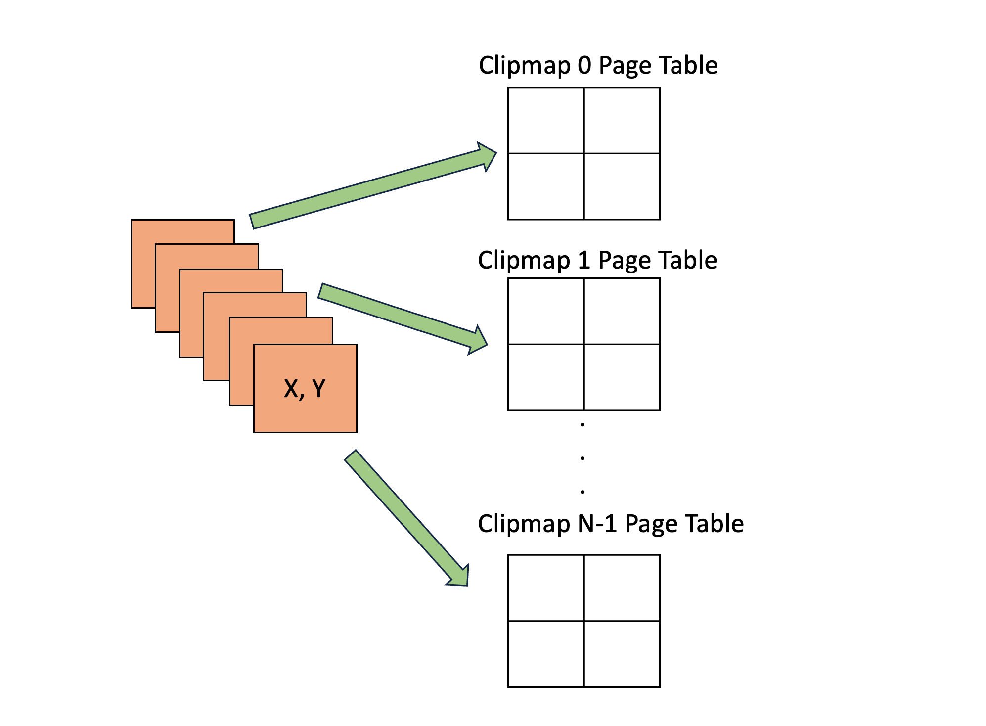
After step 1 has marked all the needed page tables for this frame, we can check each page table entry to see if extra work needs to be done such as allocation, deallocation or marking for rendering. Each clipmap will have its own page table since each clipmap has access to the full virtual shadow map resolution. For example, if we decide we want to use 8K x 8K resolution with 6 clipmap, we will have 6 8K x 8K virtual textures which are allocated from a shared physical memory pool.
If the virtual page is already backed by a valid piece of physical memory that is up to date, no further processing is needed.
If the virtual page does not have a valid page table entry or the data is out of date, this represents a page fault. At this point two things are needed. The first is to mark that page table entry as dirty so that future parts of the pipeline know to render shadows for this piece of the scene. The second is that if we cannot reuse existing physical memory, we need to write some information into the CPU readback buffer to let it know that it needs to allocate some new physical memory for the GPU to use.
Step 3: Handle Page Faults, Clear Memory
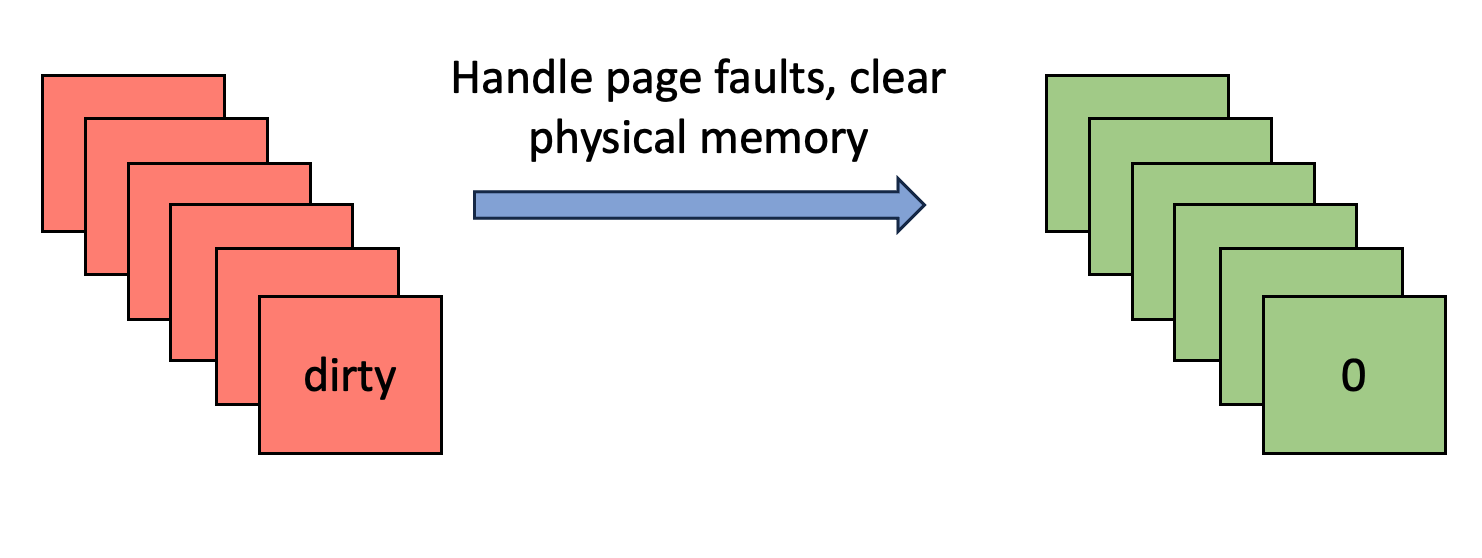 If there are any memory allocation/deallocation requests, this is something that the CPU needs to help the GPU with. On the CPU side this pseudocode represents what it needs to do with the readback:
    allocDeallocRequests = readback.MapMemory();
    for each request
        if request.xy < 0 then deallocate page
        else allocate page
With this setup, if the GPU wrote a negative page coordinate to the buffer it is asking for it to be deallocated. Positive page coordinates are allocation requests.
Once there is valid memory, control can be returned to the GPU so that it can clear all dirty pages since they are now backed by physical memory.
Note: It is possible to reduce the need for most readback situations if a full (or close to full) GPU-driven SVSM implementation is used. In this scenario the physical backing memory is a fixed size 2D texture pool pre-allocated during initialization and made available to shaders with a bindless approach. The GPU can then manage its own allocations.
Step 4: Compute Screen Bounds
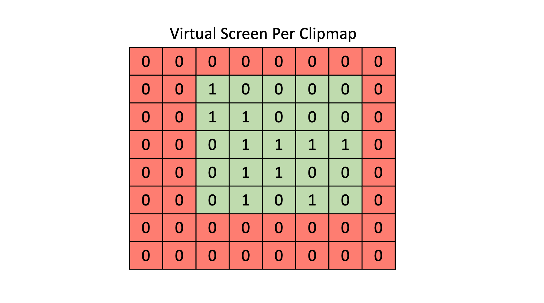
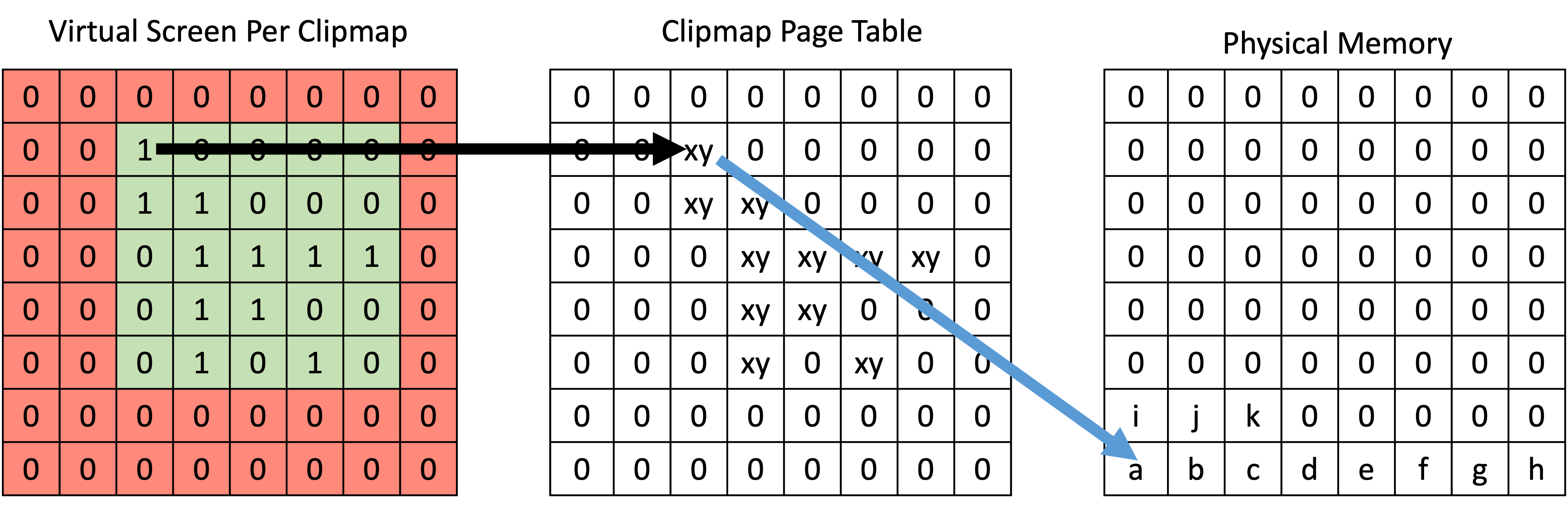
Each cascade will have its own ViewProjection matrix for rendering, and this means that it can be represented as a virtual screen. For each virtual pixel we can map it to a page table entry, check if that entry is dirty and if so, that portion of the virtual screen needs to be rendered. At the end we will have a set of screen tiles (each as large as a page) that need to be rendered. In the picture this region of screen tiles that need to be rendered is green while everything in red can be skipped.
You’ll notice that some pages marked 0 are included in the page bounds. This represents some degree of wasted effort, but for simplicity the renderable screen region is made rectangular. Object culling can help with this situation since it can reduce or eliminate fragments being generated for screen tiles that are within the update region but don’t need to be updated.
Step 5: Cull Objects
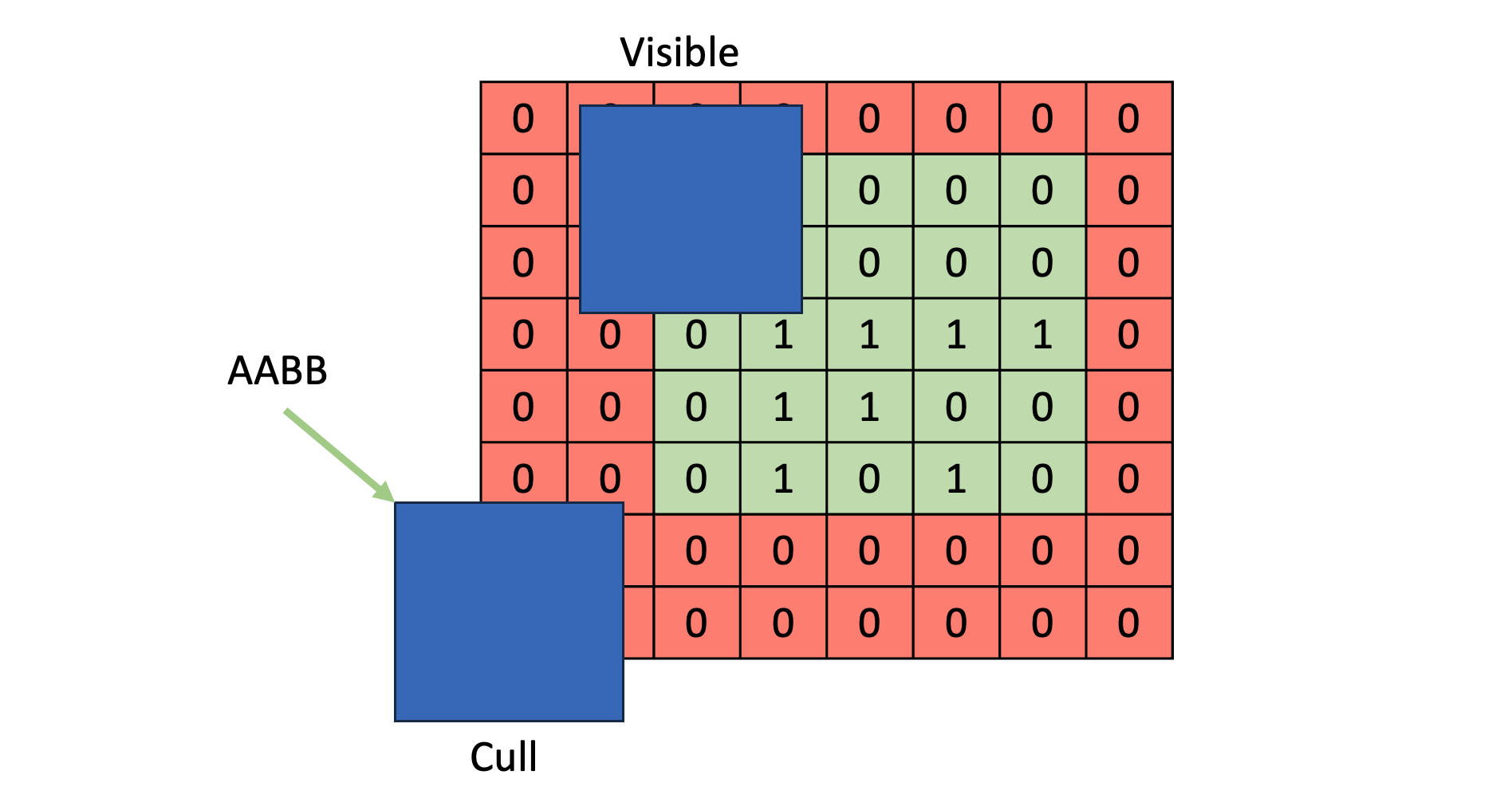
Using the screen bounds computed in step 4, objects can be culled per clipmap. To do this project their AABBs into NDC space using the render ViewProjection matrix for each clipmap. This will give better-than-nothing results. Better results can be gained by using a hierarchical culling structure based on depth or based on information about residency/cache status from the page table. A hierarchical depth structure can be used to determine if an object is likely occluded by another object, while a hierarchical page structure can be used to determine if an object overlaps one or more resident yet uncached pages.
Step 6: Render To Physical Memory
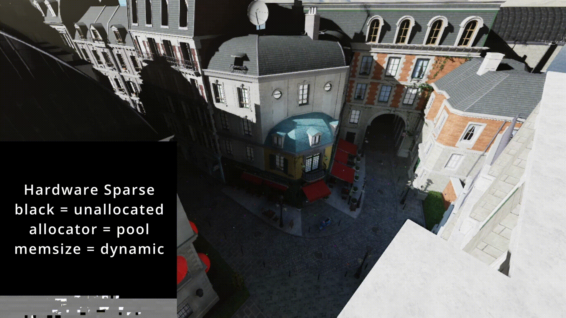
There are two ways to render the shadow map depending on the approach you take (software sparse vs hardware sparse). The difference is that with software sparse the application performs all memory management manually whereas with hardware sparse the driver tracks all memory residency and can perform optimizations not possible with software sparse.
The first method is to do a manual depth write to the physical texture. This can be used with both software sparse or hardware sparse, but it has the unfortunate side effect of disabling early z fragment discard. To do this the physical backing texture is bound as a 32-bit unsigned integer image to the fragment stage which should be one of the supported format conversions from 32-bit float. This will give access to image atomics which are only guaranteed to be available for signed and unsigned integer types. The fragment shader can then be given a set of virtual uv coordinates and a depth value. The depth value for the fragment is first converted to its representation in bits using something like floatBitsToUint. From here it will translate the virtual uv coordinates to physical uv coordinates and then perform an imageAtomicMin operation to write the depth.
The second method becomes available if using hardware sparse and requires API and driver support (more on this later). If you opt to make each shadow’s texture a hardware-managed sparse texture, you can use that as a framebuffer depth render target. This will mean that instead of using image atomics you can allow the hardware to write the depth value itself like with normal rendering. With this approach, early z fragment discard becomes available once again. With hardware sparse all resident and non-resident pages are tracked by the driver and it can automatically discard any fragments that fall within non-resident pages.
This is the end of the high level overview of the virtual shadow rendering pipeline. The rest of the article will go into more specific details about certain technical aspects of the implementation and also go over some of the difficulties that are encountered.
Modifying Virtual Viewport Matrices
Helpful Resource:
Note: Depending on how good your object culling is, this might not be needed. What it does is help reduce the size of viewport that is being rendered to in order to offset any false positives that the culling algorithm produces. The less false positives there are, the less there is a need for viewport bounds changes. However, it could still be useful as a tool for implementing per-frame shadow render budgets by only updating parts of the virtual viewport and saving the rest for later.
We can augment each clipmap’s ViewProjection matrix to only encompass the screen bounds computed in step 4. This will enable us to render the part that changed and skip what didn’t much more effectively. To do this the matrix can be split into tiles and fractionally translated so that we can set the viewport size to be exactly the step 4 bounds.
If we have a page table that is 64x64, this means we also have 64x64 screen tiles. NDC space goes from [-1, 1] meaning it is 2 units wide, high and deep. This means each tile is 2/64 = 1/32 units in size. What we can do is sum up the number of tiles we want to render in the X and Y directions and merge them into larger groups. Here is some pseudocode that will do that:
    // Index of the min and max screen tiles we want to render
    ivec2 minScreenTilesXY = minimum from step 4;
    ivec2 maxScreenTilesXY = maximum from step 4;

    ivec2 screenTileRange = maxScreenTilesXY - minScreenTilesXY;

    // Merge them into larger screen tile groups
    vec2 newNumScreenTiles = vec2(totalNumScreenTilesXY) / vec2(screenTileRange);

    // Convert minimum screen tiles to [0, 1] range
    vec2 normalizedScreenTiles = vec2(minScreenTilesXY) / vec2(totalNumScreenTilesXY);

    // Translate the normalized screen tiles into fractional locations within
    // the new merged screen tiles
    vec2 newMinScreenTilesXY = normalizedScreenTiles * newNumScreenTiles;
Once we’ve done this, the last part is to augment our ViewProjection matrix with a scale and translate identical to the way this link describes.
    vec2 inverseXY = 1.0 / newNumScreenTiles;

    float tx = - (-1.0f + inverseXY.x + 2.0f * inverseXY.x * newMinScreenTilesXY.x);
    float ty = - (-1.0f + inverseXY.y + 2.0f * inverseXY.y * newMinScreenTilesXY.y);

    mat4 scale(1.0f);
    MatScale(scale, vec3(newNumScreenTiles, 1.0f));

    mat4 translate(1.0f);
    MatTranslate(translate, vec3(tx, ty, 0.0f));

    mat4 newProjectionViewRender = scale * translate * clipmap[i].ProjectionViewRender();
Now for rendering this clipmap, newProjectionViewRender is used. This will save on a lot of performance because we can set the viewport bounds to be only the area of the virtual screen that changed.
Mapping Virtual Memory to Physical Memory
Page Table Structure
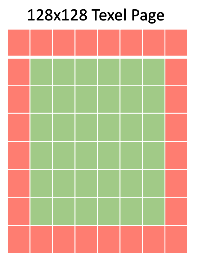
Each entry in the page table manages the state for a single 128x128 texel page. So, if the virtual resolution is set to 8182x8192, the page table will need to be 64x64 elements in size.
Here is a possible implementation of a page table entry (32 bits per entry):
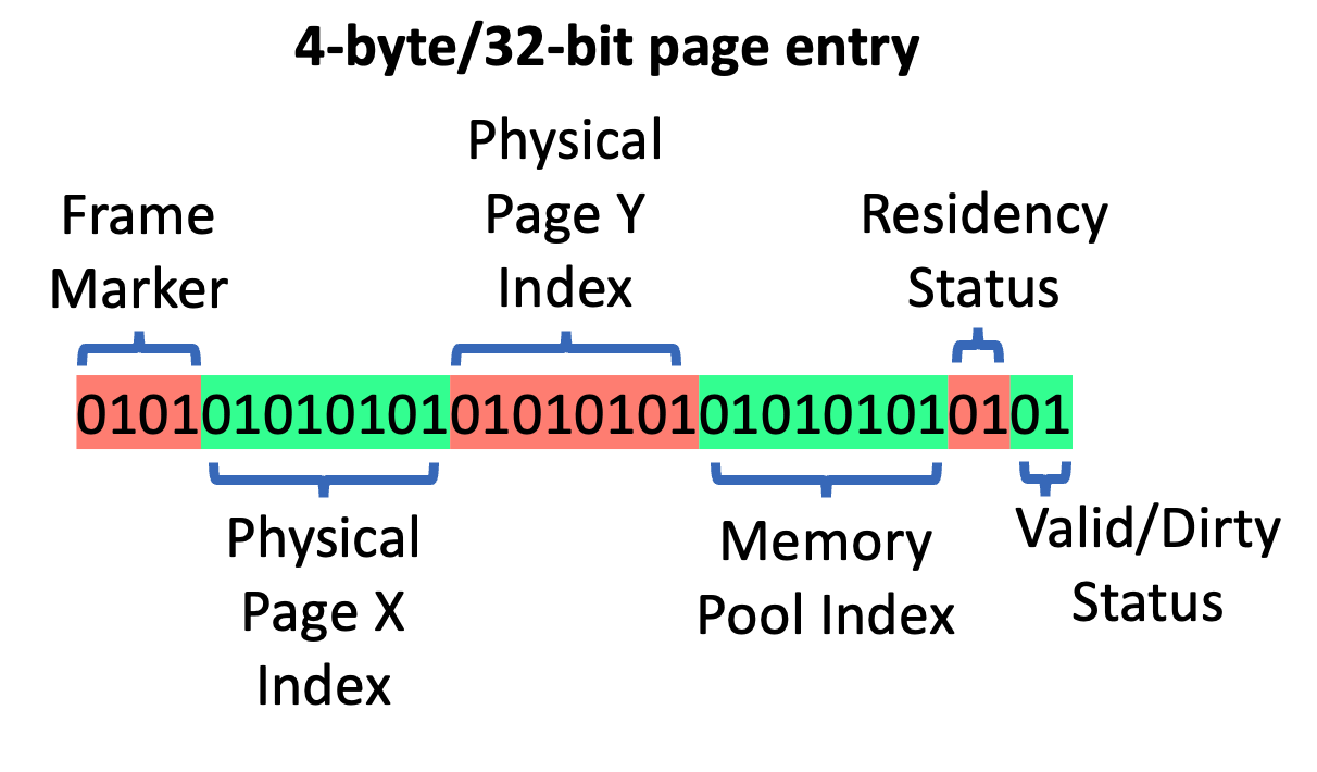
Frame Marker: Used for marking the page table entry as in use. 0 means unmarked, 1 means marked this frame, and anything greater than 1 means it was marked a few frames ago but is not currently needed for this frame. This is useful if you want to add a slight frame delay before evicting something from the cache.
Physical Page Index X/Y: Points to the lower-left corner of the physical page in memory. Reconstructing the lower-left physical texel from the page index is done using Physical Page Index X/Y * ivec2(128) where 128 represents texels per page in the x/y direction.
Memory Pool Index: This technique works by allocating physical memory from a series of either sparse or shared texture memory pools. In the case of sparse textures, the API allows for making pages resident or non-resident and doing sparse texture binding. In the case of shared texture memory, fixed-size textures are allocated from and returned to the shared texture pool as needed. The memory pool index can either refer to the array index (when using sparse texture arrays) or the texture index (when using separate textures pulled from a shared pool).
Residency Status: Tells the allocator whether a page is backed by physical memory or not.
Valid/Dirty Status: This tells the renderer whether a page needs to be re-generated or not. When the clip origin shifts, pages that fall in the update region can be marked as dirty.
ClipMap Matrix Structure
At this stage we need to define a clear way of converting from world coordinates to virtual page coordinates and then to physical texel coordinates. To do this we are going to define two different groups of matrices: projection-view sample and projection-view render. Each frame the projection-view render matrix will potentially change via translation and represents the clip origin + extent, but the projection-view sample matrix will either never change or very rarely change (depending on your use case and how far the camera has moved from world origin). The sample matrix is used to get virtual uv coords that we can use to access the page table and so its origin will be set to (0, 0, 0). The render matrix is used when rendering the shadow map using normal hardware rasterization and its origin changes as the camera moves through the scene.
Once we have these two groups of matrices, the steps of moving from virtual to physical are as follows:
1) Translate local clip map uv coordinates (projection-view render) to virtual clip map uv coordinates (projection-view sample)
2) Perform coordinate wrap around for any values outside of [0, 1] range
3) Use wrapped coordinates to access the page table and pull-out physical X/Y offset and memory pool index
4) Use physical X/Y offset and memory pool index to construct physical uv coordinates
5) Access physical texture with physical uv coordinates for either sampling or writing
Projection View Sample (stable virtual addressing)
We are going to define the projection view sample matrix as being positioned at (0, 0, 0) and set up the light orthographic projection matrix as follows:
\[\begin{bmatrix} 2 / d_k & 0 & 0 & 0 \\ 0 & 2 / d_k & 0 & 0 \\ 0 & 0 & 1 / z & 0 \\ 0 & 0 & 0 & 1 \\ \end{bmatrix}\]Where \(d_k\) is the maximum view-space extent of the first clipmap and \(z\) is the maximum depth. Each clipmap after the first maintains the same maximum depth but doubles the extent (\(d_k\)). Because of this, only the first matrix needs to be passed into the shader and the rest can be derived.
The global clip origin (0, 0, 0) view-projection matrix is created by multiplying the orthographic projection above with the rotation-only directional light view matrix.
The view matrix looks like this:
\[\begin{bmatrix} a & b & c & 0 \\ d & e & f & 0 \\ g & h & i & 0 \\ 0 & 0 & 0 & 1 \\ \end{bmatrix}\]where the upper 3x3 matrix contains only rotation.
Projection View Render
All local clip origin matrices share the same orthographic matrix from above. The only difference is that they add a translation component to their local directional light view matrix. As the player moves around the scene, we want to change the clip origin so that we can render the shadows in concentric rings around the player.
The view matrix looks like this:
\[\begin{bmatrix} a & b & c & t_x \\ d & e & f & t_y \\ g & h & i & 0 \\ 0 & 0 & 0 & 1 \\ \end{bmatrix}\]The upper 3x3 matrix is identical to the one used for projection-view sample. Multiplying it with the projection matrix from above we get this:
\[\begin{align*} \begin{bmatrix} 2 / d_k & 0 & 0 & 0 \\ 0 & 2 / d_k & 0 & 0 \\ 0 & 0 & 1 / z & 0 \\ 0 & 0 & 0 & 1 \\ \end{bmatrix} \times \begin{bmatrix} a & b & c & t_x \\ d & e & f & t_y \\ g & h & i & 0 \\ 0 & 0 & 0 & 1 \\ \end{bmatrix} = \begin{bmatrix} 2a/d_k & 2b/d_k & 2c/d_k & 2t_x/d_k \\ 2d/d_k & 2e/d_k & 2f/d_k & 2t_y/d_k \\ g/z & h/z & i/z & 0 \\ 0 & 0 & 0 & 1 \\ \end{bmatrix} \end{align*}\]Now let’s see what happens when we multiply this matrix by a world space position
\[\begin{align*} \begin{bmatrix} 2a/d_k & 2b/d_k & 2c/d_k & 2t_x/d_k \\ 2d/d_k & 2e/d_k & 2f/d_k & 2t_y/d_k \\ g/z & h/z & i/z & 0 \\ 0 & 0 & 0 & 1 \\ \end{bmatrix} \times \begin{bmatrix} v_x \\ v_y \\ v_z \\ 1 \end{bmatrix} = \begin{bmatrix} 2av_x/d_k + 2bv_y/d_k + 2cv_z/d_k + 2t_x/d_k\\ 2dv_x/d_k + 2ev_y/d_k + 2fv_z/d_k + 2t_y/d_k \\ gv_x/z + hv_y/z + iv_z / z \\ 1 \end{bmatrix} \end{align*}\]This gives us NDC coordinates for the first clip map. What if we want to convert the result back to what it would have been if we had used projection-view sample? We can subtract off \(2t_x/d_k, 2t_y/dk\) from the result.
What about for the other clipmaps? We know that for each successive clip map, \(d_k\) doubles in size but everything else remains the same including the translation component. So, to convert from clipmap 0 to clipmap n, we can multiply the result by \(1/2^c\) where \(c\) is the clipmap index from [0, clipmaps - 1].
Because of this we only need to pass in the matrix for the very first clip map and we can use it in the shader to convert to any other clipmap, or back to the projection-view sample space. Here is some GLSL code that does this:
    #define BITMASK_POW2(shift) (1 << shift)

    // For first clip map - rest are derived from this
    uniform mat4 vsmClipMap0ProjectionViewRender;
    uniform uint vsmNumClipMaps;
    uniform uint vsmNumPagesXY;
    uniform uint vsmTexelResolutionXY;

    layout (r32ui) coherent uniform uimage2DArray pageTable;

    vec3 VsmConvertClip0ToClipN(in vec3 original, in int clipMapIndex) {
        vec3 result = original;
        result.xy *= vec2(1.0 / float(BITMASK_POW2(clipMapIndex)));
        return result;
    }

    // Returns values on the range of [-1, 1]
    vec3 VsmCalculateRenderClipValueFromWorldPos(in vec3 worldPos, in int clipMapIndex) {
        vec3 result = (vsmClipMap0ProjectionViewRender * vec4(worldPos, 1.0)).xyz;

        // Accounts for the fact that each clip map covers double the range of the
        // previous
        return VsmConvertClip0ToClipN(result, clipMapIndex);
    }

    // Subtracts off the scaled translate component
    vec3 VmCalculateSampleClipValueFromWorldPos(in vec3 worldPos, in int clipMapIndex) {
        vec3 result = VsmCalculateRenderClipValueFromWorldPos(worldPos, clipMapIndex);

        // Accounts for the fact that each clip map covers double the range of the
        // previous
        return result - VsmConvertClip0ToClipN(vsmClipMap0ProjectionView[3].xyz, clipMapIndex);
    }
Performing Coordinate Translation
Now we have everything we need to go from world space to virtual coordinates to physical coordinates. For a given world space coordinate, we will calculate the sample clip value and convert that to virtual texture coordinates.
    vec3 ConvertWorldPosToPhysicalCoordinates(in vec3 worldPos, in int clipMapIndex) {
        vec3 ndc = VmCalculateSampleClipValueFromWorldPos(worldPos, clipMapIndex);

        vec2 virtualTexCoords = ndc.xy * 0.5 + 0.5;

        ...
Next we need to perform coordinate wrap around. To do this we can use the fract function which computes x - floor(x).
virtualTexCoords = fract(virtualTexCoords);Next we can use these wrapped virtual coordinates to get the page table entry. Once we have that we can use bitmask operations to pull out the physical page X/Y offset and memory pool index.
ivec2 pageTableIndex = ivec2(floor(virtualTexCoords * vec2(vsmNumPagesXY)));
uint entry = imageLoad(pageTable, ivec3(pageTableIndex, clipMapIndex)).r;
ivec2 physicalPageXYOffset;
int memoryPoolIndex;
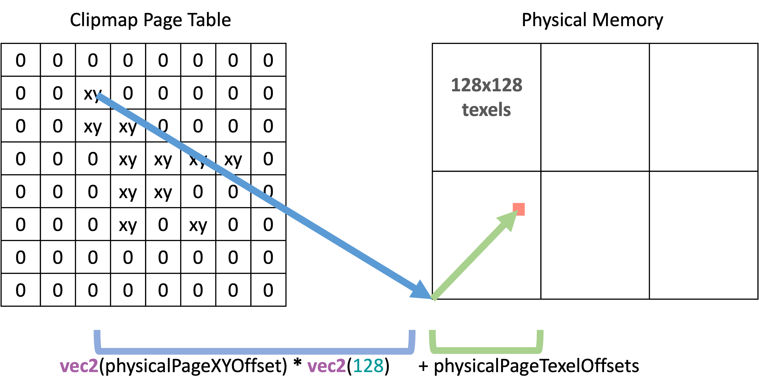
UnpackPhysicalMemoryData(entry, physicalPageXYOffset, memoryPoolIndex);Once we have these values, what we need to do is figure out which texel the virtualTexCoords are trying to point to. What we know about the physical pages is that they are 128x128 texels in size. So, to figure out which texel we need to point to, we can calculate the virtual pixel coordinate and mod it by 128.
        vec2 virtualPixelCoords = virtualTexCoords * vec2(vsmTexelResolutionXY);
        vec2 physicalPageTexelOffsets = mod(virtualPixelCoords, 128.0);
The final step is to convert these coordinates to actual physical coordinates that we can use to sample the physical texture. Since physicalPageXYOffset points to the lower-left corner of the physical page (in indices, not texels) and physicalPageTexelOffsets points to the texel within that page, we can multiply physicalPageXYOffset by the number of texels per page (128) and add it to physicalPageTexelOffsets.
        return vec3(
            vec2(physicalPageXYOffset) * vec2(128) + physicalPageTexelOffsets,
            float(memoryPoolIndex)
        );
(visual of above mapping code)
And we’re done! We now have a way to convert from world space coordinates -> virtual coordinates -> physical memory coordinates. If we revisit the rendering step 6 from above, what this means is that we will use newProjectionViewRender for each clipmap to rasterize the scene. For each fragment that we generate we want to convert it to physical coordinates and write the depth to that location.
In practice this means something like gl_Position will be written in the vertex shader using newProjectionViewRender, but it will smooth out a set of texture coordinates that it generates using ConvertWorldPosToPhysicalCoordinates with the world position. This way the fragment shader uses the smoothed in texture coordinates to write out gl_FragCoord.z to the shadow map.
Selecting Clipmaps
Given a world position, how can we quickly determine which clipmap it will fall in? We can look at the NDC output from multiplying the first clipmap’s projection view render with a world position.
\[\begin{align*} \begin{bmatrix} 2av_x/d_k + 2bv_y/d_k + 2cv_z/d_k + 2t_x/d_k \\ 2dv_x/d_k + 2ev_y/d_k + 2fv_z/d_k + 2t_y/d_k \\ gv_x/z + hv_y/z + iv_z / z \\ 1 \end{bmatrix} = \begin{bmatrix} n_x \\ n_y \\ n_z \\ 1 \end{bmatrix} \end{align*}\]Looking at the X and Y component, we know that if the world position fell within the first clipmap, the NDC will be on the range of [-1, 1]. If the result is outside of this range, it means that we need to multiply \((n_x, n_y)\) by \((1/2^{c_x}, 1/2^{c_y})\) to bring it back within the [-1, 1] range. If we can solve for positive integer values of \((c_x, c_y)\), we get back two values representing the clipmaps where this is true.
\[\begin{align*} \begin{bmatrix} |n_x| \times 1/2^{\lceil c_x \rceil} \\ |n_y| \times 1/2^{\lceil c_y \rceil} \\ \end{bmatrix} = \begin{bmatrix} 1 \\ 1 \\ \end{bmatrix} \end{align*}\]Focusing on solving for just one of them since both will be the same format:
\[\begin{aligned} & | n_x | \times 1/2^{\lceil c_x \rceil} = 1 \\ & (| n_x | \times 1/2^{\lceil c_x \rceil}) \times 2^{\lceil c_x \rceil} = 2^{\lceil c_x \rceil} \\ & | n_x | = 2^{\lceil c_x \rceil} \\ & \lceil log_2(| n_x |) \rceil = log_2(2^{\lceil c_x \rceil}) \\ & \lceil log_2(| n_x |) \rceil = {\lceil c_x \rceil} \times log_2(2) \\ & \lceil log_2(| n_x |) \rceil = {\lceil c_x \rceil} \\ \end{aligned}\]We take the ceiling of \(log_2\) on the left since otherwise it would give us fractional solutions which we don’t want here. Since this is undefined at \(n_x=0\) and \(log_2(1)=0\) (first clipmap index), we can constrain \(n_x\) using max.
\[\begin{aligned} & \lceil log_2(max(| n_x |, 1)) \rceil = {\lceil c_x \rceil} \end{aligned}\]This is the solution for \(n_x\), but \(n_y\) will also give us a value. When there is a situation where the two results are different, the largest will be the correct answer. Here is some GLSL code:
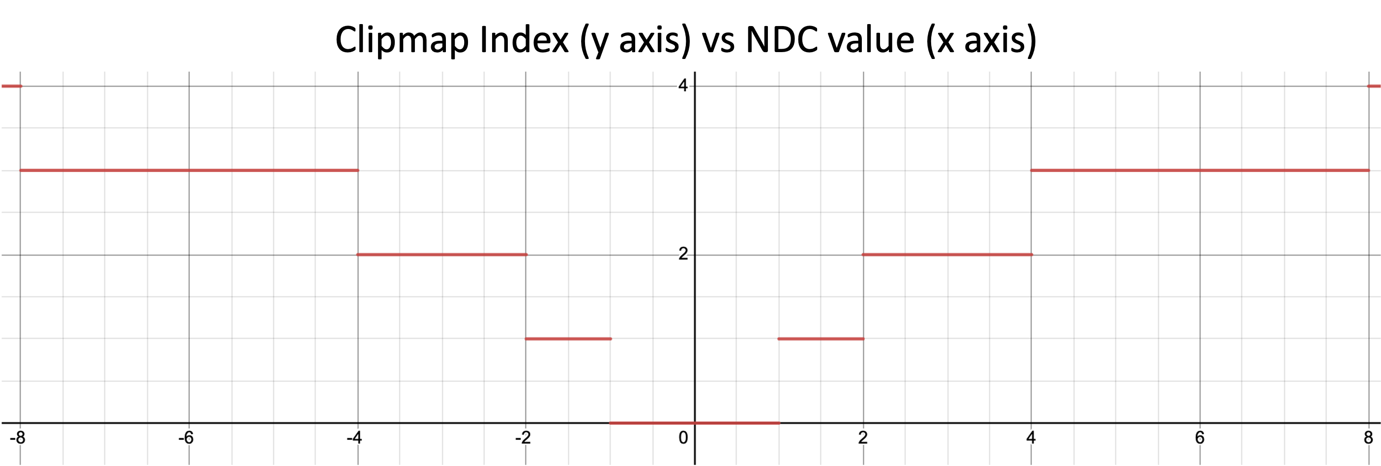
int VsmCalculateClipmapIndexFromWorldPos(in vec3 worldPos) {
    // Get the normalized device coordinates (NDC) for the first clipmap
    vec2 ndc = VsmCalculateRenderClipValueFromWorldPos(worldPos, 0).xy;

    vec2 clipmapIndex = vec2(
        ceil(log2(max(abs(ndc.x), 1))),
        ceil(log2(max(abs(ndc.y), 1)))
    );

    return int(max(clipmapIndex.x, clipmapIndex.y));
}
Here is a graph of the above function to show how the clipmap index changes as the NDC value changes.
Here is a visual of clipmap changing as the camera moves closer or further from geometry:

When pages become visually smaller and change in color tone this is an indication they are part of finer clipmaps. Visually larger pages are an indication they are part of coarser clipmaps.
Cache Invalidation Events
There are a few situations where one or more cache entries become invalid. The first is the most common which is when a page is no longer needed for the current frame. In this case it can be marked invalid and its physical memory freed up for other pages.
Light Rotation
Another common situation is when the directional light rotates. This is a case when projection-view sample changes, and because of this the entire virtual address mapping changes.
This situation results in all the pages becoming invalid at the same time. If the light is rotating very slowly it may be possible to reuse old data while staggering the updates to improve performance, but this is an open issue I don’t have a good answer to right now. One approach mentioned in this Fortnite article is that if your scene will have frequent directional light changes, fine tune shadow rendering to prioritize page rendering performance. One way would be reducing the virtual resolution: drop down to 8K or 4K. Another is to adopt a meshlet-based rendering pipeline to reduce the number of pages each object overlaps (improves culling potential). Another is to avoid doing a continuous rotation and instead split it into several incremental rotations so that the shadow updates can be spread out over multiple frames.
Here is a visual of the location of the pages changing because of directional light rotation:
Dynamic Objects
Another event resulting in cache invalidations is when objects in the scene move around. There are at least two approaches to dealing with this. The first is to render static and dynamic objects into the same clipmaps. When an object moves its AABB could be used to check which pages it overlaps with and then mark those as invalid.
The second is to maintain two sets of clipmaps: one for static objects and one for dynamic objects. Dynamic object clipmaps can be tailored towards being updated almost entirely every frame whereas static objects can use the incremental update approach as the camera moves.
Allocation Strategy
An easy way to handle allocation for this virtual memory system is to pack a list of free pages into a shader storage buffer object (SSBO). When the GPU wants to allocate, it can remove the topmost entry using shader atomics and add that page to the corresponding page table entry. When it wants to deallocate, it can add the page back to the front of the list again using shader atomics. With this system the GPU will add pages back to the free list whenever its page table frame marker exceeds some value less than the max supported by the frame marker bits.
Another option would be to implement a cache using one a replacement policy such as least recently used (LRU). More cache replacement policies can be found on this Wikipedia article.
In the following gif the lower left shows the first memory pool as it pulls pages from the free list or adds them back. Black = unallocated.
Hardware/API Sparse Memory
OpenGL, Vulkan and DirectX all have dedicated API support for hardware sparse memory allocation.
The main issue is that even though these are supported, there have been reports of major issues with performance especially on Windows. For example:
Your mileage may vary and will require profiling for the target hardware and OS/drivers.
Software Sparse Memory
In the absence of good support for hardware/API sparse memory, the main alternative is to fallback to regular textures and texture arrays. Each texture will have a fixed power of 2 size and be capable of representing some number of physical 128x128 texel pages. These textures can be allocated from and returned to a shared texture memory pool as needed.
Allocation Strategy Comparison
Hardware sparse leverages driver/API sparse memory management+binding support. Software sparse manages memory manually and allocates from fixed-size texture pools.
Physical Memory Limits
Each implementation will need to decide how to deal with the case of a memory pool running out of memory during a given frame. It’s possible that more pages will be requested than a single memory pool can handle. One approach would be to trigger a page fault like normal, then allow the CPU to allocate a whole new block to pull memory from. For example, say each pool is a 1024x1024 2D texture (8 pages x 8 pages). If that pool runs out, the CPU could reserve another 1024x1024 pool and begin allocating from that. This could continue until some maximum upper bound is reached (either configued by the app or dictated by available VRAM). It would also be an option to later free that texture pool if none of the pages from it are currently referenced.
Another approach would be to have a fixed-size texture pool that never grows or shrinks and evict pages corresponding to coarser clipmaps and prioritize putting them in the clipmaps closer to the camera. This would mean that if the current frame runs out of physical memory, it could rebalance the pages that will be rendered based on which ones are the highest priority (finer clipmaps) vs lower priority (coarser clipmaps).
Another approach would be to process each clipmap separately all the way through final shading by selecting the clipmap, allocating memory, rendering shadows, shading, moving to next clipmap. This could be very difficult to optimize the performance of, but it would guarantee that each clipmap would have access to all available physical memory if required. It would look something like:
1) Preprocess: Analyze depth and mark pages required for all clipmaps
2) Select clipmap
3) Allocate memory for any requested pages in (1) that aren’t already backed by phyiscal memory
4) Render shadows for uncached pages
5) Perform shading on any parts of the scene covered by this clipmap
6) Go back to (2) for next clipmap
Shadow Render Budget
One possible performance optimization is to add a configurable render budget for shadow map generation. To conceptualize this, we can return to the clip map page from earlier.
From this image we can see that each clipmap, even though not strictly part of a mip chain, can still be used as one since each successive clipmap is fully capable of representing everything from the previous clipmap, just at a lower effective resolution.
This allows us to specify one or more clipmaps to serve as the lowest/coarsest levels in the mip chain. When we perform the depth buffer analysis, not only will we mark the pages in the finest detail mip levels, but we will also mark the corresponding pages in the lowest mip levels.
Then what we can do when rendering is to set a budget for how many pages from the finest mips to process before saving them for the next frame. The lowest mips will be rendered fully every frame so we can use them as a fallback when data is not available at a higher resolution.
This gif shows what this looks like (slowed down to exaggerate the shadow pop in):
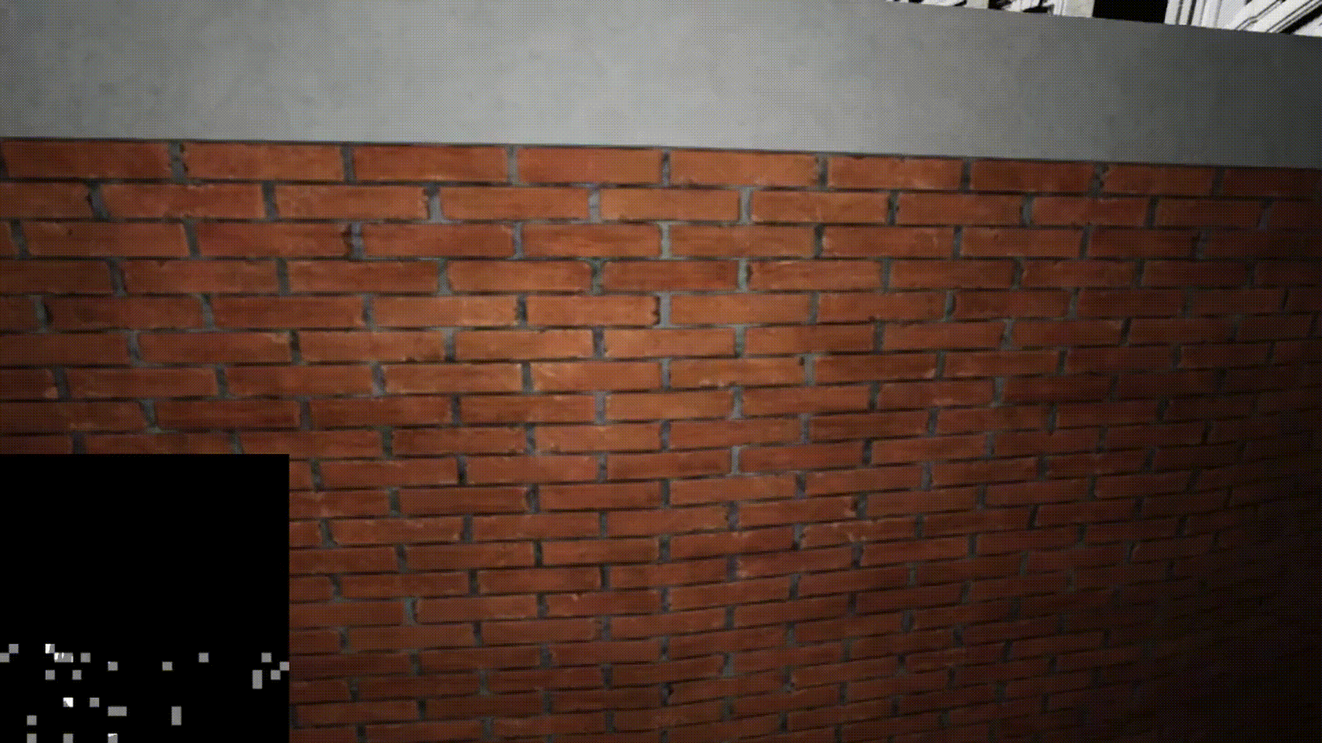
As the camera moves through the wall, you’ll notice that part of the scene must temporarily fall back to lower (coarser) mip levels until all of the higher (finer) mip levels are processed.
This is a nice option to have since it provides a setting that can be tweaked for different hardware and different scene complexities. It could also be set dynamically to help when the rendering is struggling to maintain target frame times.
Hardware Shadow Filtering
An issue comes up when we try to use hardware shadow filtering such as with sampler2DShadow. For most of the texels within a page the hardware can freely perform its filtering without issue, but the problem is at the page border:
Everything in the green represents texels that won’t cause an issue with hardware shadow filtering. Everything in the red is where the problems start since the hardware will assume it can sample into the next adjacent pages. But the next pages will almost always contain data from completely different parts of the scene.
Option 1: Border
For this option you can contract or expand the size of the shadow map so that you can add a 1 texel border around each page. Then it is possible to use hardware filtering without any issues or having to handle special cases.
Option 2: Hybrid
Another option is to write a sampling function that checks to see if the starting texel is on the page boundary. If it is, you can perform software shadow filtering so that you can avoid sampling into memory that has nothing to do with the current page.
If not on a border, use hardware filtering as normal.
Option 3: Manual
The last option is to abandon hardware shadow filtering completely and write your own software filtering code. This has the advantage of not requiring branching in the shader or adding any page borders.
Post-Processing Effects
There will be times when certain post processing effects such as volumetric lighting might require data to be present in the shadow map that is outside of the current view of the camera. When this is the case, it will be necessary to add some extra logic during the page marking/depth prepass stage. The clipmap that is marked will depend on what level of resolution the post processing effect will need. If it can get away with low resolution, then it can go with the further/coarser clipmaps to save on bandwidth and performance.
Thanks for reading!
References
- Virtual Shadow Maps in Unreal Engine
- Virtual Shadow Maps in Fortnite Battle Royale Chapter 4
- The Clipmap: A Virtual Mipmap
- Sparse Virtual Textures
- Another Sparse Virtual Textures
- Understanding Virtual Memory
- Terrain Rendering Using GPU-Based Geometry Clipmaps
- Fitted Virtual Shadow Maps
- Queried Virtual Shadow Maps