StratusGFX Technical Frame Analysis
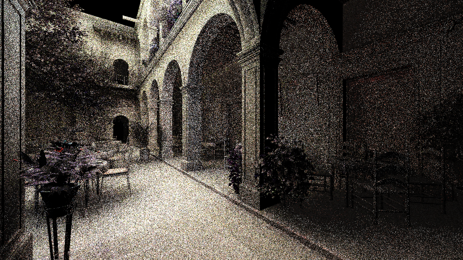
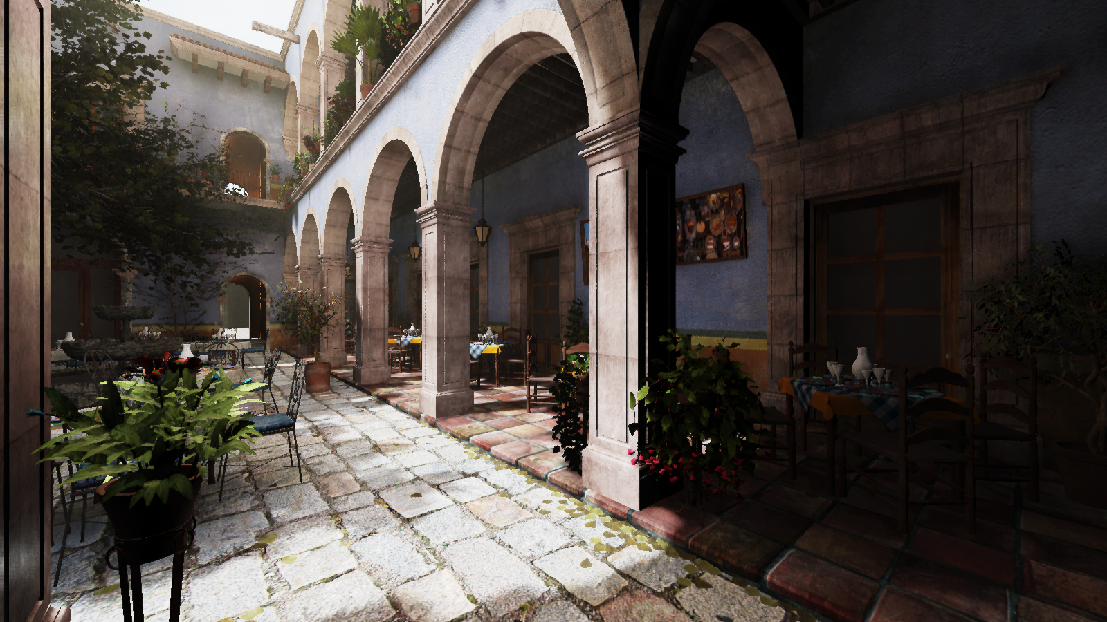 (rendered with StratusGFX v0.10 - model is San Miguel)
This article will breakdown a lot of the high level technical details of how the Stratus graphics engine v0.10 renders a single frame. It is designed to be a deferred renderer with minimal forward passes. For performance it attempts to make heavy use of async data streaming to improve load times, reuses data from previous frames when it can, and amortizes work over the course of many frames.
All scenes have been rendered in realtime on an Nvidia GTX 1060.
Table of Contents
- Table of Contents
- How A Frame Is Rendered
- Async Model and Texture Loading
- Entity and Light Changes
- Shader Recompile
- GPU View Frustum Culling & Mesh LOD Selection
- Cascaded Shadow Maps (CSMs)
- Shadow Map Cache and Updates
- GBuffer (Geometry Buffer) Generation
- Physically Based Direct Lighting (Metallic-Roughness Pipeline)
- Screen Space Ambient Occlusion
- Realtime Global Illumination
- Raymarched Volumetric Lighting and Shadowing
- Anti-Aliasing: FXAA + TAA
- Bloom
- Final Result
- A Few Other Sample Scenes
- References
How A Frame Is Rendered
The graphics engine uses a GPU-driven pipeline that makes heavy use of programmable vertex pulling, multi-draw indirect and bindless resources. This allows for just a few large GPU buffers to be used to store all mesh data, material data and draw indices that all draw commands can reference. The draw commands themselves are stored in GPU memory meaning that the GPU itself can generate and modify its own draw commands that will later be submitted to the render queue.
Bindless resources mean that the renderer can determine at the start of the frame which textures need to be used (shadow maps, diffuse maps, normal maps, etc.) and ensure that they are all made resident on the GPU before any draw calls are made. The material data buffer contains handles that are used to reference these resident textures.
This GPU-driven, bindless pipeline allows for another optimization technique known as draw call merging. For example, the renderer can batch up all commands that have similar render settings into one command buffer and then dispatch them with a single multi-draw indirect call. This also makes it possible to cache previously generated command buffers and reuse them in future frames if nothing has changed.
Another interesting opportunity is also created by using this approach. Since all materials and their textures are made resident at the start of the frame, any shader at any stage can access any material property or texture that they might need without having to add in new C++ code to make them available to that shader. This makes adding new shaders that work on different parts of the data very easy.
This technique is used by id Tech 7 and can be read about here: https://advances.realtimerendering.com/s2020/RenderingDoomEternal.pdf
A lot of this is also covered in the “3D Graphics Rendering Cookbook” and “OpenGL SuperBible 7th Edition”.
Async Model and Texture Loading
First the resource manager checks if during the last frame any model or textures have finished loading. These assets are streamed in asynchronously by worker threads. When their data has finished being loaded and processed, the resource manager uses the renderer thread to copy the finalized data into the relevant GPU buffers.
To enable meshes to be better processed by multiple threads and to help the renderer with things like fine grained frustum culling, meshes are split into smaller submeshes or meshlets. Each submesh contains no more than 4096 polygons and has its own bounding box.
Entity and Light Changes
The next thing the renderer does is to do a check over entities and lights marked “dynamic” to see if any of them have changed within the last frame or if new ones have been added. The reason this is done is for two reasons:
1) If no entities have been changed or added, previous render queues may be entirely valid for this new frame and can be reused.
2) If a light has not moved or had an entity move near it, its shadow map data from the previous frame can be reused.
Anything marked as static is skipped during this step to save on performance.
Shader Recompile
Next up is a check to see if the application code has requested a shader recompile. If so all shaders are marked as invalid and the latest code is loaded from disk and compiled.
This capability was added very early in development and having it saved tons of time. A lot of shader effects were written and debugged while the engine was running.
GPU View Frustum Culling & Mesh LOD Selection
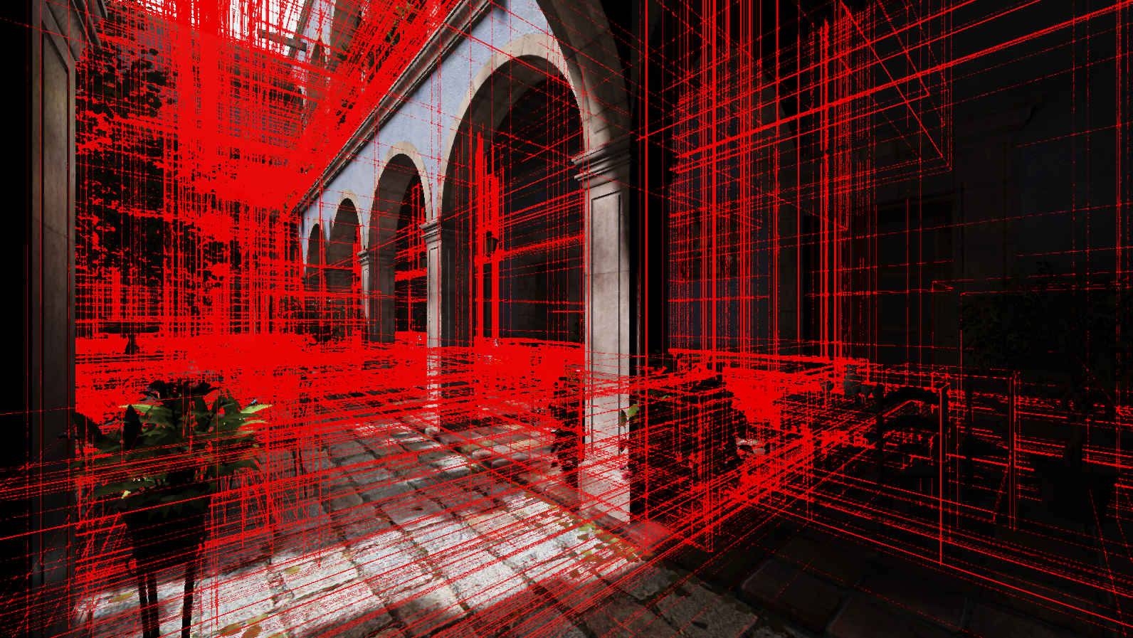 (Visual of the scene’s submeshes by overlying their AABBs onto the scene)
The CPU then dispatches a compute shader which is responsible for culling draw commands by performing a visibility test of its Axis-Aligned Bounding Box (AABB) against the view frustum.
If a command passes the view frustum test meaning the mesh it represents is at least partially inside the frustum, the compute shader then checks to see how far away in view space that mesh is. Based on the distance it decides which LOD should be used, and finally writes the command to a GPU draw command buffer.
If a command fails the view frustum test meaning it’s fully outside at least one of the frustum planes, the GPU marks that command as unnecessary by setting its instance count parameter to 0.
Cascaded Shadow Maps (CSMs)
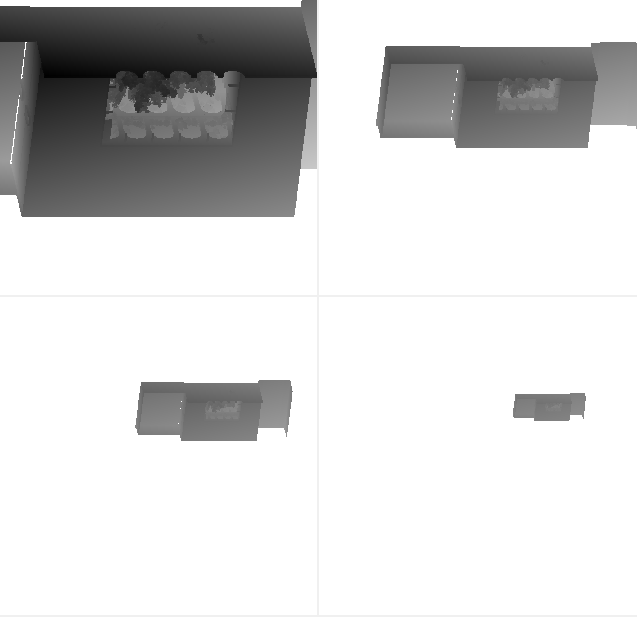
(Shadow map cascades 1 (top left), 2 (top right), 3 (bottom left), 4 (bottom right))
The current setting is for the view frustum to be split into 4 regions using the practical split scheme. To help with performance, the first two cascades are rendered with the LODs that were selected during the view frustum culling and LOD select stage. The last two cascades use the lowest LOD available which at the time of writing is LOD 8.
In order to try and deal with shadow aliasing/artifacting a few techniques are used. These are:
- Render the shadow maps with reverse face culling enabled
- Render the shadow maps with hardware slope-based depth biasing
- Per-app configurable software depth bias
- Apply an offset to the position used to sample the shadow map based on the surface normal and light direction
With tweaks to these techniques it is possible to get some pretty good results even with relatively low resolution shadow maps.
Shadow Map Cache and Updates
All local lights pull from a set of large shadow map atlases which serve as a shadow cache. Each atlas can store the shadow data for up to 300 separate lights and atlas entries are reused heavily between frames.
If a light changes, it is entered into a queue which is processed incrementally over many frames. This prevents performance from falling apart when many lights change at once.
As new lights are streamed in while the camera moves around the world, old lights are evicted from the atlas if there are no free entries. Old data is then overwritten with the data for the new lights that have come into view.
Finally, if a light hasn’t changed and its data is still valid in the shadow map cache, that data will be reused without change.
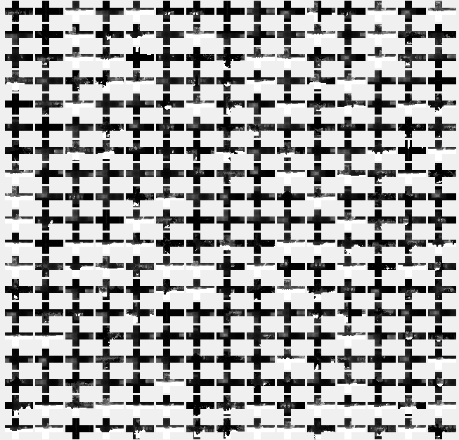
(View of one of the shadow map atlases with data from many different lights)
GBuffer (Geometry Buffer) Generation
Now the GBuffer is generated so that it can be used with the deferred lighting and post processing passes. World space positions are reconstructed from the depth value so an explicit world space texture is not used. These are the following textures that are part of the GBuffer for this implementation:
1) 8-bit RGB world space normal texture (converted from tangent space -> world space)
(It was pointed out to me that GBuffer normals can be handled more efficiently. See here: https://aras-p.info/texts/CompactNormalStorage.html)
2) 8-bit RGBA albedo texture with emissive.r in the alpha channel
3) 8-bit RG Reflectance texture (f0) with emissive.g in the green channel
4) 8-bit RGB Roughness-Metallic texture with emissive.b in the blue channel
5) 16-bit RGBA Structure buffer
6) 16-bit RG Velocity buffer
Used for effects such as TAA and temporal accumulation of indirect illumination.
7) 32-bit R Mesh Draw ID buffer
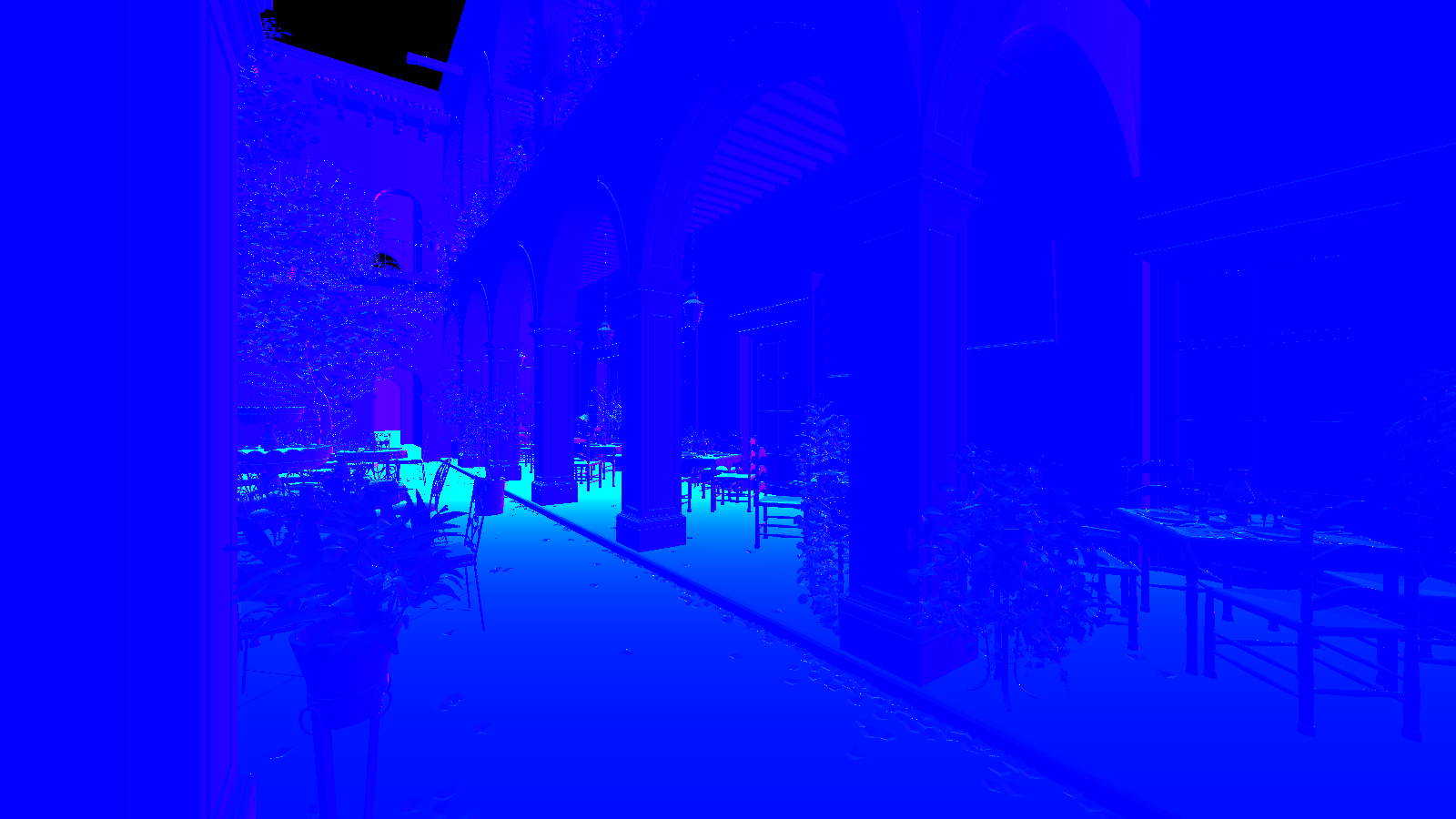 (Structure buffer)
The structure buffer is composed of three elements:
- Partial derivative of camera-space depth with respect to current x window coordinate
- Partial derivative of camera-space depth with respect to current y window coordinate
- Camera-space depth
The partial derivatives are calculated by the fragment shader using the dFdx and dFdy functions in GLSL: https://registry.khronos.org/OpenGL-Refpages/gl4/html/dFdx.xhtml
This buffer is used for effects such as SSAO and volumetric lighting.
 (Mesh Draw ID buffer)
This buffer enables post processing to see which mesh a pixel represents by storing its ID. This is used for things like detecting disocclusion events when dealing with passes that perform temporal data reuse such as TAA or denoising.
Physically Based Direct Lighting (Metallic-Roughness Pipeline)
The current PBR implementation for this engine is based on the PBR paper released by Google’s Filament team. This can be found here: https://google.github.io/filament/Filament.md.html.
Right now the standard model single scattering bidirectional reflectance distribution function (BRDF) is used by the engine so it will unfortunately lose energy at high roughness values. The diffuse term is using the Disney model since I liked the results a bit better even though it cost a tiny bit of performance.
At this stage only direct and local lights are processed. Since global illumination is enabled, no fixed ambient term is required.
Screen Space Ambient Occlusion
This implementation is based on the SSAO chapter found in “Foundations of Game Engine Development, Volume 2: Rendering”.
This algorithm runs in two passes. The first pass builds a buffer which represents how much ambient light reaches a given surface. If the value is low the result is less ambient light for that pixel. To build this buffer, a fragment shader samples the structure buffer in 4 places around the current pixel. What it is trying to do is use the structure buffer’s information to figure out if there is nearby geometry that is occluding ambient light that would otherwise be reaching the current surface. The 4 places that the fragment shader reads from are randomly offset by a 4x4 rotation texture that we precompute on the CPU. This rotation texture is set up and used in such a way that for every 4x4 group of nearby pixels, their structure buffer sampling patterns will amount to 64 unique samples.
The second pass is to perform depth-aware blurring to try and smooth out artifacts such as dotted patterns which tend to appear.
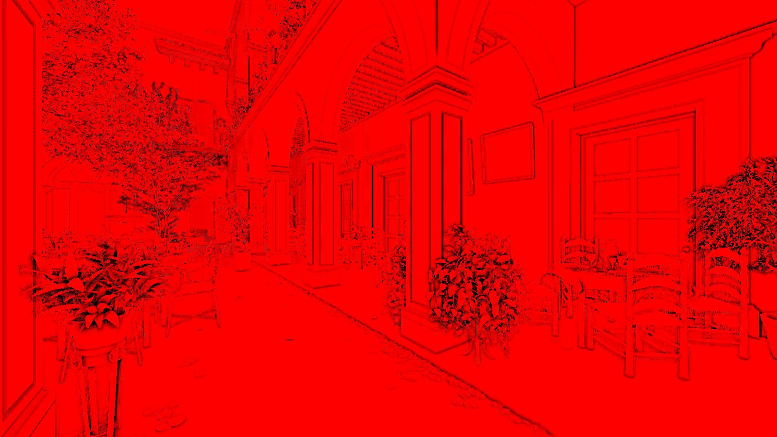
(SSAO buffer)
Once this is complete it can be passed into the global illumination pipeline.
Realtime Global Illumination
Second bound indirect illumination (diffuse+specular+occlusion) is handled by using virtual point lights (VPLs) which are spread around the scene. Each one captures some local lighting information and is then used to transfer radiance to other surfaces that weren’t hit by direct lighting.
A 3rd indirect bounce is not directly simulated but shadows are tapered to prevent harsh cutoff.
While many VPLs can exist in the scene, only 4200 of the nearest VPLs are considered per frame. This number could be lowered for hardware less powerful than a GTX 1060 or raised for more powerful hardware that has extra vram. The VPLs are first selected as candidates by the CPU and a GPU compute stage narrows it down to 4200 or less by testing the VPLs against the cascaded shadow maps. In shadow means that VPL is not visible and therefore does not contribute to the indirect illumination.
For each pixel an adaptive sampling approach is used. A number of samples between 1 and 10 are selected based on the surface’s distance to the camera and whether or not its lighting history was recently discarded due to a disocclusion event (recently discarded = temporarily sample more heavily).
To estimate occlusion a technique called imperfect shadow maps are used. With this a low resolution representation of the screen is rendered into a very low resolution shadow map representing a VPL. This is combined with SSAO from the previous step to try and approximate occlusion of indirect lighting.
Here is the result:
(Adaptive sampling of VPLs at each pixel)
Since the result is very noisy the next step is to denoise. This is done with two approaches. The first is inspired by ReSTIR and involves allowing each pixel to look at its neighbors. If that neighbor is a good fit geometrically and spatially, it is able to probabilistically merge that neighbor’s samples into its own to increase the effective sampling count without having to actually compute more samples per pixel.
This clears up a lot of the noise but not all. To finish the denoising a 2-level wavelet denoiser inspired by SVGF is used and its results are temporally accumulated meaning it reuses data from previous frames. This is the result:
(Denoised indirect illumination without textures)
It’s important that denoising happens before textures are applied or else it would end up blurring out a lot of important texture details. By decoupling indirect illumination from the texture detail you prevent blurry visuals while still maintaining high-quality denoised indirect lighting.
Finally, denoised lighting data is recombined with the textures. This is the result:
Raymarched Volumetric Lighting and Shadowing
This implementation is based on the atmospheric shadowing chapter found in “Foundations of Game Engine Development, Volume 2: Rendering”.
The purpose of this step is to simulate how light interacts with participating media, which could be things like water vapor or dust particles. These are the high level details of the model used here:
1) Some fraction of light traveling through the air will be redirected towards the camera (inscattering)
2) Some fraction of the light traveling through the air will be redirected away from the camera (outscattering and backscattering)
3) Some will be absorbed by the participating media and not reach the camera (extinction)
4) Some is occluded completely due to a distant object blocking rays of light.
The result of this is that parts of the scene will appear foggy or hazy while still allowing the viewer to see through to the other side. When there are distant objects blocking light rays, there will be noticeably darker areas in the fog which give the appearance of light rays/God rays (also known as crepuscular rays). This is very noticeable when in a forested scene or when light is streaming through a window but is partially blocked by the central frame.
This Digital Foundry video explains it very well: https://www.youtube.com/watch?v=G0sYTrX3VHI.
To accomplish these effects the renderer performs raycasting in camera space and uses the cascaded shadow maps combined with the structure buffer. For each pixel, one ray is cast and sampled along 64 non-linear locations (exact sampling count configurable at runtime). The sampling density is highest at points along the ray closest to the camera and sparsest at points that are furthest away from the camera. We end the sampling early if the ray runs into some geometry which is checked by using the structure buffer.
For each sampling step, if that location is not in shadow after checking it against the cascaded shadow maps, it applies a fog model which estimates how much light is inscattered towards the camera based on the current distance along the ray. If it is in shadow that sample is skipped. These steps are accumulated into a final value per pixel which can be blended with the main screen texture.
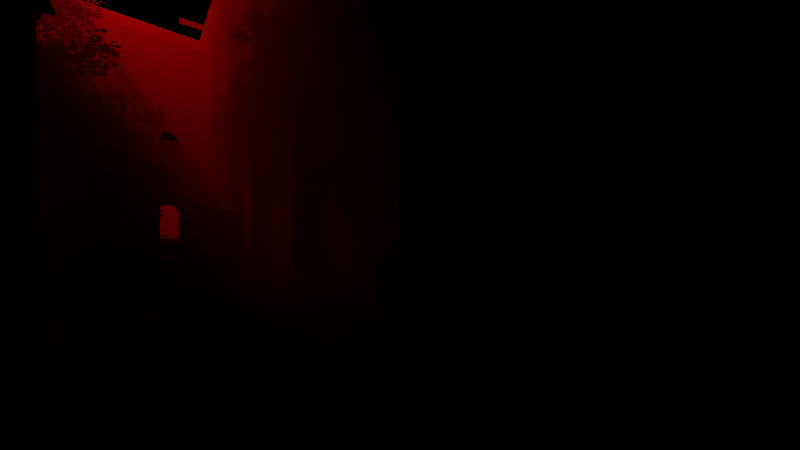
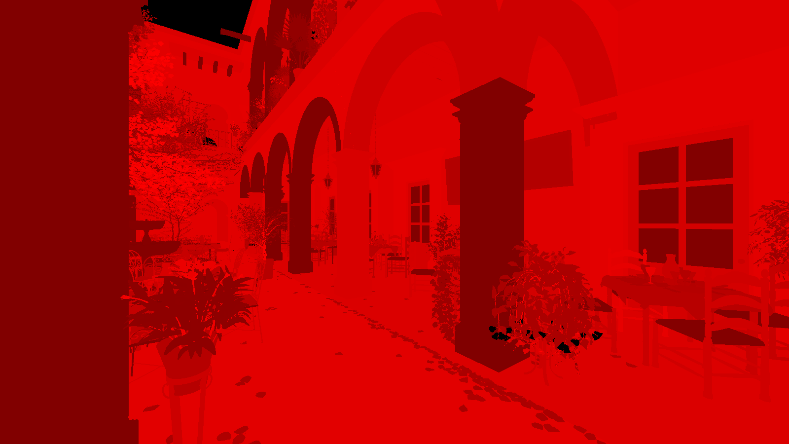
(Volumetric lighting buffer - values exaggerated to show contrast)
This buffer is then combined with the rest of the scene to give the appearance of volumetric lighting and shadowing.
Anti-Aliasing: FXAA + TAA
There are two anti-aliasing algorithms currently implemented. By default they both operate together but it is possible to enable just one or the other or disable both. These two algorithms are Fast Approximate Anti-Aliasing (FXAA) and Temporal Anti-Aliasing (TAA).
TAA
The first stage is to apply TAA at the beginning of the post processing pipeline. This works by rendering each frame with a slightly different subpixel offset to create subpixel jitter. The offsets are pulled from the first 16 elements of the base-2, base-3 Halton sequence. This results in 16 frames each with slightly different geometry positions which can then be blended together (temporal blending) in order to produce a softer image.
Since this happens before the rest of the PostFX pipeline such as bloom, it first needs to tonemap the values it gets from HDR to LDR before applying the temporal blending. In order to try and prevent lag and ghosting, the color blend is clamped between the minimum and maximum color values of the neighbors around the current pixel. This means that when the color in the history buffer is too high or too low based on the current neighborhood, the history buffer is rejected for that pixel.
Once this is done it inverse tonemaps the result from LDR back to HDR so that the rest of the post FX pipeline can run.
FXAA
After tonemapping and gamma correction at the end of the PostFX pipeline, FXAA is applied. This is done using a non-linear series of steps to identify edges and apply blurring. A final guess step is taken if the end of the edge was not found within 10 steps. For more information see https://catlikecoding.com/unity/tutorials/custom-srp/fxaa/.
Bloom
Next it moves onto physically based bloom. In order to accomplish this it first highlights bright parts of the scene and writes them into their own separate buffer, then it progressively downsamples the buffer followed by progressive upsampling. This blurs all of the bright parts of the scene which can then be merged with the main image. The result is that very bright regions end up looking as if the light is bleeding outwards slightly into nearby darker areas.
For more information on this technique you can check out the Call of Duty: Advanced Warfare presentation.
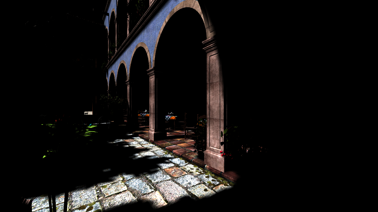
Final Result
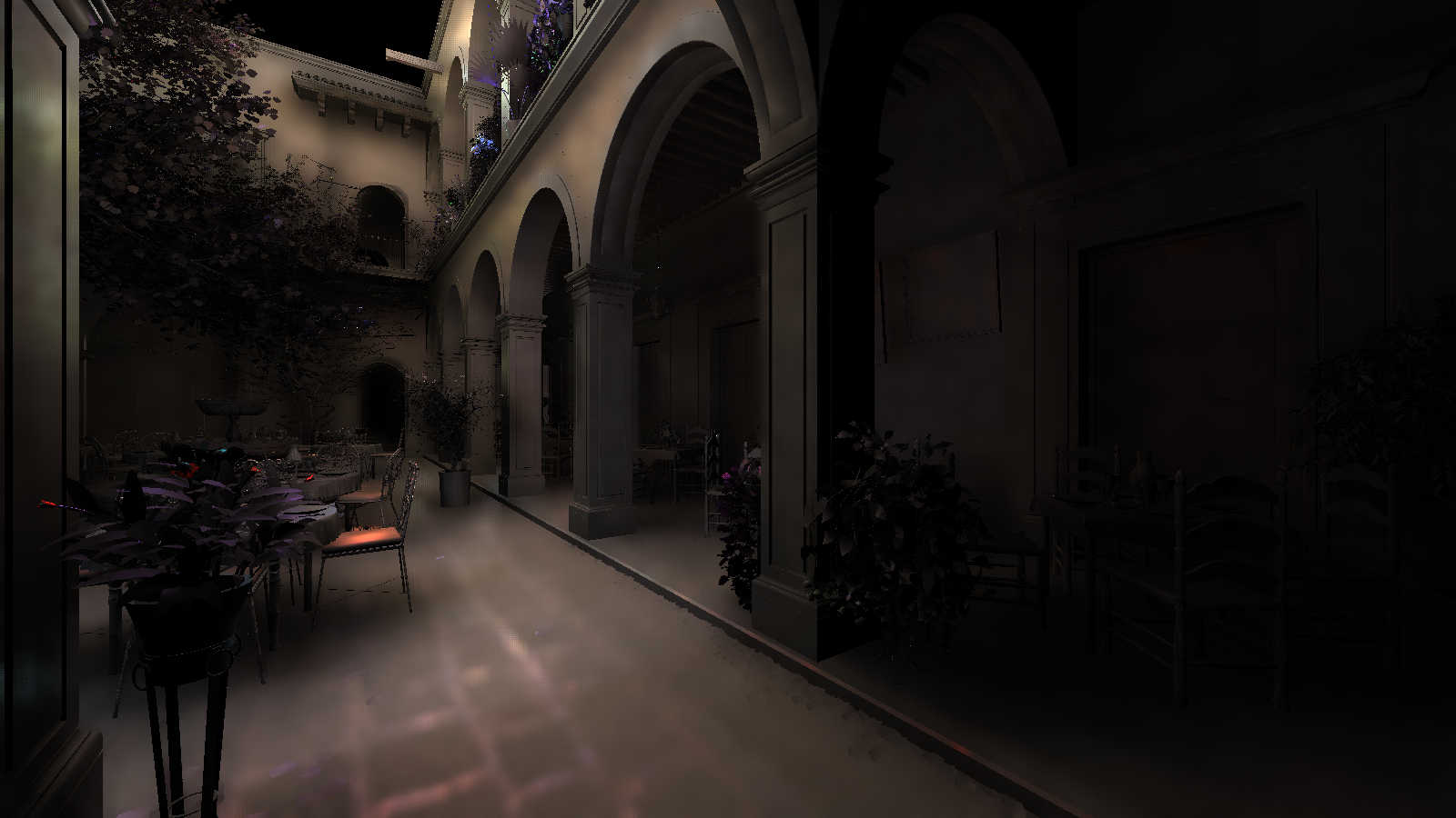
After all the post FX has completed including gamma correction and ACES tonemapping, this is the result:
A Few Other Sample Scenes
Each was rendered with v0.10 of the engine.
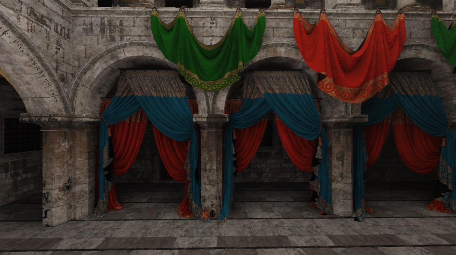
(3D Model: Intel Sponza)
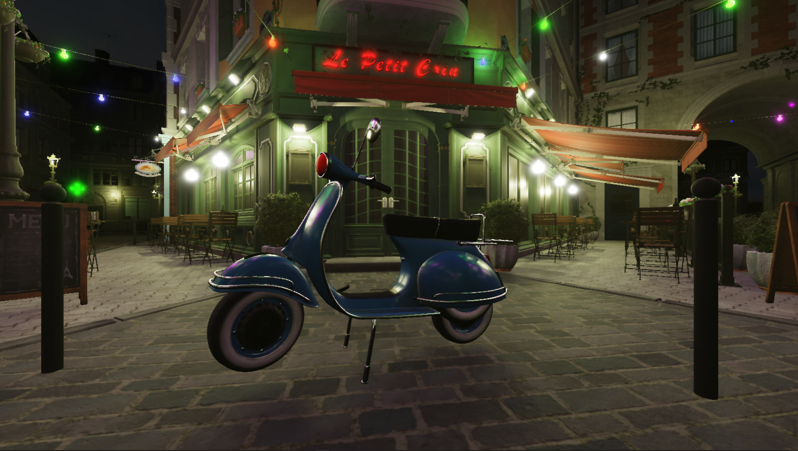
(3D Model: Amazon Lumberyard Bistro)
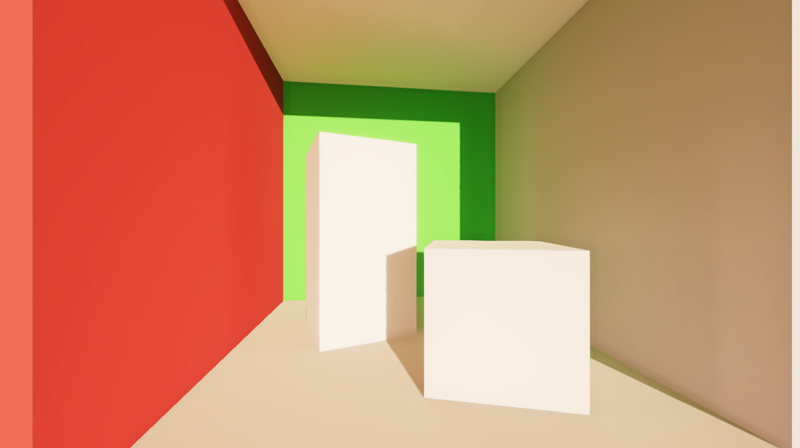
(3D Model: Cornell Box)
References
General
- https://learnopengl.com
- 3D Graphics Rendering Cookbook
- OpenGL SuperBible
- Foudations of Game Engine Development, Volume 1: Mathematics
- Foundations of Game Engine Development, Volume 2: Rendering
- Physically Based Rendering Online Book
- Game Engine Architecture
- Biskwit’s YouTube Channel
- Cem Yuksel’s YouTube Channel
- Fabien Sanglard’s Website
- https://advances.realtimerendering.com/s2020/RenderingDoomEternal.pdf
Physically Based Rendering
Global Illumination
- Imperfect Shadow Maps
- SVGF
- ASVGF
- Q2RTX Real-Time Path Tracing and Denoising
- Q2RTX + Albedo Demodulation
- Reconstruction Filters
- SVGF Presentation
- ReSTIR
- ReSTIR Math Breakdown
- ReSTIR Theory Breakdown
- Global Illumination in Tom Clancy’s The Division
- Interactive Graphics 22: Global Illumination
- Radiance Caching for Real-Time Global Illumination
Cascaded Shadow Maps
Temporal Anti-Aliasing
- https://sugulee.wordpress.com/2021/06/21/temporal-anti-aliasingtaa-tutorial/
- https://ziyadbarakat.wordpress.com/2020/07/28/temporal-anti-aliasing-step-by-step/
- https://www.elopezr.com/temporal-aa-and-the-quest-for-the-holy-trail/
- http://extremelearning.com.au/unreasonable-effectiveness-of-quasirandom-sequences/
- https://de45xmedrsdbp.cloudfront.net/Resources/files/TemporalAA_small-59732822.pdf